3. Random- and Fixed-Effects Models (Week 4 - Part I)

Key Concepts

• Random-Effects Model - Allows the inclusion of intact groups (clusters) within a model
  • Each cluster is given its own random intercept made up of its mean and its residual variance, meaning that each group has a different, or random, intercept
• Intraclass Correlation (ICC) - A ratio that indicates the percent of variation in the outcome that is attributed to the group. It represents between-group differences.
  • The inverse is attributable to individual- or lowest-level differences
  • The way variance is partitioned is a good indicator of homogeneity of individuals on the outcome
    • Low ICC means less differences among groups and more differences among individuals within groups, meaning individuals are independent of each other
    • High ICC means more difference among groups than within them, meaning individuals within groups are interdependent.
• Fixed-Effects Model - Allows for the inclusion of a dummy variable that controls for group-level effects

Success for All (SFA) Program

The following example comes from Murnane and Willett (2010), chapter 7. The data was originally downloaded from the UCLA Institute for Digital Research and Education (IDRE).

The data examines a subset of SFA data which focuses on first graders in their first year in which their school participated in the SFA program. The example focuses on a single outcome, a “Word-Attack” reading test score measured at the end of the first year.

# load packages
library(tidyverse)
library(haven)
library(psych)
library(apaTables)
library(gt)
source("data/apafunction.R")

#load data
wattack <- read_dta("data/methods_matter/ch7_sfa.dta")

Variables:

• schid: school ID
• stuid: student ID
• wattack: Word Attack reading score
• sfa: treatment = 1, control = 0
• ppvt: pretest score
• sch_ppvt: school average of ppvt pretest score

Descriptive Statistics

Overall

describe(wattack$wattack) %>%
  as.data.frame() %>%
  select(n, mean, sd, min, max, skew, kurtosis) %>%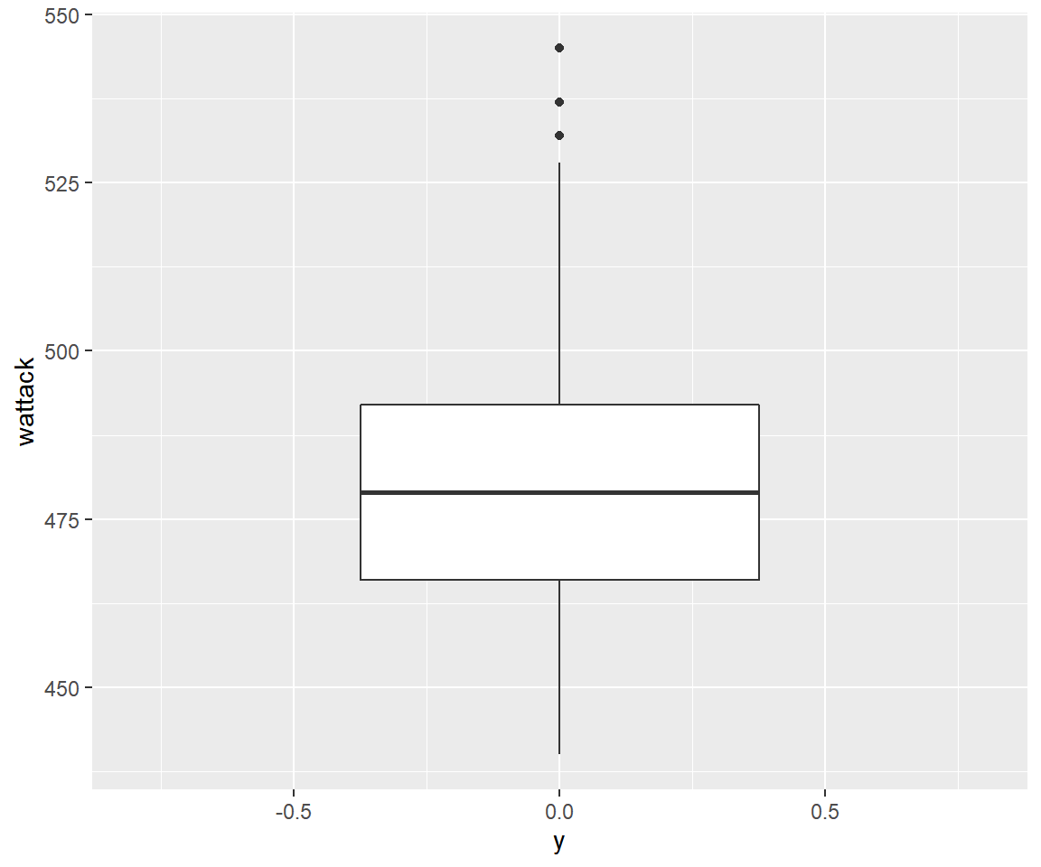
  apa()

n	mean	sd	min	max	skew	kurtosis
2334	478.5193	19.87872	440	545	-0.1653687	-0.2012883

Box Plot of Word Attack Scores (overall)

wattack %>%
  ggplot(aes(wattack)) +
  coord_flip()+
  geom_boxplot()+
  expand_limits(y=c(-.8,.8))

Descriptive Statistics of Word Attack Score by School

wattack %>%
  group_by(schid) %>%
  summarize(mean = mean(wattack),
            sd = sd(wattack),
            min = min(wattack),
            max = max(wattack),
            "Freq." = n()) %>%
  rename("School ID" = schid) %>%
  head(n=5) %>% #show only 5
  apa("Descriptive statistics of Word Attack score by school (first 5 schools)")

Descriptive statistics of Word Attack score by school (first 5 schools)
School ID	mean	sd	min	max	Freq.
1	475.7308	16.15988	440	519	52
2	486.6034	15.31063	449	532	116
3	491.3676	16.84690	449	532	68
4	462.9118	16.55179	440	494	34
5	495.0851	14.96783	464	532	47

wattack %>%
  ggplot(aes(wattack, y=as.factor(schid))) +
  coord_flip()+
  geom_boxplot()

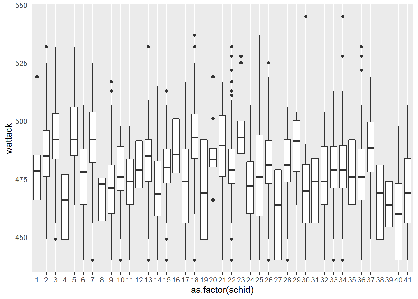
Note

The above boxplot shows the between-school variability and is similar to visualizing the intraclass correlation.

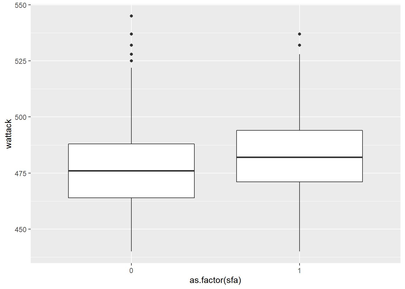
Descriptive Statistics by Experimental Condition (sfa)

wattack %>%
  group_by(sfa) %>%
  summarize(mean = mean(wattack),
            sd = sd(wattack),
            min = min(wattack),
            max = max(wattack),
            "Freq." = n()) %>%
  rename("Condition" = sfa) %>%
  apa("Descriptive statistics of Word Attack score by school (first 5 schools)")

Descriptive statistics of Word Attack score by school (first 5 schools)
Condition	mean	sd	min	max	Freq.
0	474.8247	20.05239	440	545	1118
1	481.9161	19.10511	440	537	1216

wattack %>%
  ggplot(aes(wattack, y=as.factor(sfa))) +
  coord_flip()+
  geom_boxplot()

Models

Instructions from

• https://rpubs.com/rslbliss/r_mlm_ws
• https://rpsychologist.com/r-guide-longitudinal-lme-lmer

Model 1 - Unconditional Model, Table 7.1, pg. 114

To estimate a random-effect or multi-level model, we can use lmer() from the lme4 package. We will use icc() from the performance package and r.squaredGLMM from the MuMIn package.

The function and argument is as follows:

lmer(dv ~ 1 (for unconditional) + (1 (for random) | grouping variable), data = data object)

Note: you would use (0 | grouping variable) for fixed effects.

library(lme4) # for multilevel modeling
library(performance)
library(broom) # making a table from model

# model 1
model1 <- lmer(wattack ~ 1 + (1 | schid), data=wattack)

# model table
tidy(model1) %>%
  add_row(term = "R2", 
          estimate=MuMIn::r.squaredGLMM(model1)[,1]) %>%
  add_row(term = "ICC", 
          estimate =performance::icc(model1)$ICC_adjusted) %>%
  mutate(across(is.numeric, round, 3)) %>%
  apa("Model 1 - Fitted Random-Effects Multilevel Models: Unconditional Model") %>%
  fmt_missing(
    columns = 2:5,
    missing_text = ""
  )

Model 1 - Fitted Random-Effects Multilevel Models: Unconditional Model
term	estimate	std.error	statistic	group
(Intercept)	477.535	1.451	329.137	fixed
sd_(Intercept).schid	8.896			schid
sd_Observation.Residual	17.725			Residual
R2	0.000
ICC	0.201

\(WATTACK_{ji} = (\gamma_0 + u_j) + \epsilon_{ij}\)

Interpretations

• intercept represents the grand mean of Word Attack scores across all schools
  • sd_(Intercept).schid - The residual variation for schools.
• sd_observation.Residual - The residual variation for students.
• Residuals, \(R^2\), and ICC serve as baselines of comparison across the models

Other R Functions

For other important model statistics, you can use:

• parameters::p_value() - to get p-values
  • Note: You can alos use the package lmerTest, which gives p-values but then cannot be transformed into a table
  • This is on purpose: https://link.springer.com/article/10.3758/s13428-016-0809-y
• lme4 can easily be transformed into a table with broom::tidy, broom::augment, and broom::glance but lmerTest cannot.
• performance::icc() to get the intraclass correlation
• VarCorr() - to get residual the standard deviations +tidy(model)[row,2]$estimate^2 to get the variances

Model 2 - Conditional model that contains the main effect of SFA, Table 7.1, pg. 114

# model 2
model2 <- lmer(wattack ~ sfa + (1 | schid), data=wattack)

# model table
tidy(model2) %>%
  add_row(term = "R2", 
          estimate=MuMIn::r.squaredGLMM(model2)[,1]) %>%
  add_row(term = "ICC", estimate = performance::icc(model2)$ICC_adjusted) %>%
  mutate(across(is.numeric, round, 3)) %>%
  apa("Model 2 - Fitted Random-Effects Multilevel Models: with SFA") %>%
  fmt_missing(
    columns = 2:5,
    missing_text = ""
  )

Model 2 - Fitted Random-Effects Multilevel Models: with SFA
term	estimate	std.error	statistic	group
(Intercept)	475.302	2.035	233.616	fixed
sfa	4.366	2.844	1.535	fixed
sd_(Intercept).schid	8.700			schid
sd_Observation.Residual	17.727			Residual
R2	0.012
ICC	0.194

\(WATTACK_{ji} = (\gamma_0 + u_j) + \gamma_1SFA_j + \epsilon_{ij}\)

Interpretations

• intercept - The mean word attack score across schools in the control group
• sfa - The impact of being in the SFA program on school Word Attacks scores (these schools had scores 4.366 points higher)
• sd_(Intercept).schid - The residual for schools - This has decreased to some extent as sfa accounts for some of the variation
• The treatment effect explained 6.3%, a reduction in variance.SFA accounts for 6.3% of the 20% (ICC) between schools.

• ((8.896^2)-(8.72))/(8.8986^2)

• sd_observation.Residual - Residual variation for children remains the same, as SFA is a school-level variable
• ICC has decreased somewhat and indicates the variation between schools is less when sfa is taken into account.
  • sfa accounts for 3.5% of the variance between schools
    • \(\frac{.194-.201}{.201} = -.035\)

Model 3 - Conditional model that adds the main effect of covariate SCH_PPVT to Model #2, Table 7.1, pg. 114

# model 3
model3 <- lmer(wattack ~ sfa + sch_ppvt + (1 | schid), data=wattack)

# model table
tidy(model3) %>%
  add_row(term = "R2", 
          estimate=MuMIn::r.squaredGLMM(model3)[,1]) %>%
  add_row(term = "ICC", estimate = performance::icc(model3)$ICC_adjusted) %>%
  mutate(across(is.numeric, round, 3)) %>%
  apa("Model 3 - Fitted Random-Effects Multilevel Models: with SFA and pretest scores") %>%
  fmt_missing(
    columns = 2:5,
    missing_text = ""
  )

Model 3 - Fitted Random-Effects Multilevel Models: with SFA and pretest scores
term	estimate	std.error	statistic	group
(Intercept)	419.807	12.643	33.205	fixed
sfa	3.569	2.356	1.515	fixed
sch_ppvt	0.623	0.141	4.425	fixed
sd_(Intercept).schid	7.024			schid
sd_Observation.Residual	17.725			Residual
R2	0.082
ICC	0.136

\(WATTACK_{ji} = (\gamma_0 + u_j) + \gamma_1SFA_j + \gamma_2SCH_PPVT_j + \epsilon_{ij}\)

Interpretations

• intercept - The mean of word attack scores across schools in the control group, controlling for school average pretest scores
• sfa - The impact of being in the SFA program on school Word Attacks scores, controlling for pretest scores (these schools had scores 3.569 points higher)
• sch_ppvt - school pre-test scores - these are included for statistical control and not generally needed for interpretation
• sd_(Intercept).schid - The residual for schools - This has decreased to some extent as sfa and sch_ppvt accounts for some of the variation
• The percent difference between Model 2 and Model 3 is 35%, which means school pre-test scores explains 35% of variation across word attack scores above and beyond what the treatment explains. This creates a more precise estimate in the treatment variable.
• sd_observation.Residual - Residual variation for children remains the same, as SFA is a school-level variable
• ICC has decreased somewhat and indicates the variation between schools is less when sfa and sch_ppvt are taken into account.

Model 4 - Model #3 using the within-school averages of prior ppvt score (new variable schavgppvt) from the analytic subsample instead of sch_ppvt. (Not shown in text, this analysis is mentioned in footnote 15 on page 127.) - from UCLA

# model 4
model4 <- lmer(wattack ~ sfa + schavgppvt + (1 | schid), 
               data=wattack %>%
  group_by(schid) %>%
  mutate(schavgppvt = mean(ppvt))) # mean of pretest as covariate

# model table
tidy(model4) %>%
  add_row(term = "R2", 
          estimate=MuMIn::r.squaredGLMM(model4)[,1]) %>%
  add_row(term = "ICC", estimate = performance::icc(model4)$ICC_adjusted) %>%
  mutate(across(is.numeric, round, 3)) %>%
  apa("Model 4 - Fitted Random-Effects Multilevel Models: with SFA and subsample of pretest scores") %>%
  fmt_missing(
    columns = 2:5,
    missing_text = ""
  )

Model 4 - Fitted Random-Effects Multilevel Models: with SFA and subsample of pretest scores
term	estimate	std.error	statistic	group
(Intercept)	421.604	11.690	36.064	fixed
sfa	3.216	2.323	1.384	fixed
schavgppvt	0.602	0.130	4.636	fixed
sd_(Intercept).schid	6.888			schid
sd_Observation.Residual	17.725			Residual
R2	0.086
ICC	0.131

Model Notes

This model includes within-school averages of pre-test scores rather than all pre-test scores. This variable normalizes within-school variation and thus accounts for between-school variation in a different way. Intercept is not adjusted adjusted for school differences

Schavppvt acts as a type of fixed effect (e.g. holding within-school averages constant) as it acts as a kind of grouping variable that serves to group individuals by school.

Model Variations

The following models show various ways of controlling for individual- and school-level ppvt. None of the models shown below are displayed in the text. These are from the UCLA website.

Controlling for individual-level ppvt, deviated from the grand mean (new variable ppvt_devgm).

# get grand mean
summary(wattack$ppvt)

##    Min. 1st Qu.  Median    Mean 3rd Qu.    Max. 
##    40.0    81.0    90.0    90.4   100.0   144.0

# model 5
model5 <- lmer(wattack ~ sfa + ppvt_devgm + (1 | schid), 
               data=wattack %>% 
  mutate(ppvt_devgm = ppvt-90.4)) #pre-test minus grand mean

# model table
tidy(model5) %>%
  add_row(term = "R2", 
          estimate=MuMIn::r.squaredGLMM(model5)[,1]) %>%
  add_row(term = "ICC", estimate = performance::icc(model5)$ICC_adjusted) %>%
  mutate(across(is.numeric, round, 3)) %>%
  apa("Model 5 - Fitted Random-Effects Multilevel Models: Controlling for individual-level ppvt") %>%
  fmt_missing(
    columns = 2:5,
    missing_text = ""
  )

Model 5 - Fitted Random-Effects Multilevel Models: Controlling for individual-level ppvt
term	estimate	std.error	statistic	group
(Intercept)	475.907	1.645	289.228	fixed
sfa	3.440	2.301	1.495	fixed
ppvt_devgm	0.485	0.028	17.446	fixed
sd_(Intercept).schid	6.920			schid
sd_Observation.Residual	16.725			Residual
R2	0.153
ICC	0.146

Model Notes

This model includes ppvt_devgm, which is a variable in which individual pre-test scores are centered around the grand mean. This changes the meaning of the intercept to one that is adjusted for school-level differences and refers to someone with the control group and

Controlling for individual-level ppvt by including deviations of individual scores from school-average scores (new variable ppvt_devsm) and school-average scores from the grand mean (new variable schavgppvt_devgm).

# model 6
model6 <- lmer(wattack ~ sfa + ppvt_devsm + schavgppvt_devgm + (1 | schid), 
               data=wattack %>% 
                 group_by(schid) %>%
  mutate(schavgppvt = mean(ppvt)) %>% # school average
    ungroup() %>%
    mutate(
         ppvt_devsm = ppvt-schavgppvt, # individual deviation from school average
         schavgppvt_devgm = schavgppvt-90.4)) # school average deviation from grand mean

# model table
tidy(model6) %>%
  add_row(term = "R2", 
          estimate=MuMIn::r.squaredGLMM(model6)[,1]) %>%
  add_row(term = "ICC", estimate = performance::icc(model6)$ICC_adjusted) %>%
  mutate(across(is.numeric, round, 3)) %>%
  apa("Model 6 - Fitted Random-Effects Multilevel Models: Controlling for individual-level ppvt") %>%
  fmt_missing(
    columns = 2:5,
    missing_text = ""
  )

Model 6 - Fitted Random-Effects Multilevel Models: Controlling for individual-level ppvt
term	estimate	std.error	statistic	group
(Intercept)	476.063	1.658	287.088	fixed
sfa	3.189	2.322	1.373	fixed
ppvt_devsm	0.479	0.028	16.840	fixed
schavgppvt_devgm	0.603	0.130	4.643	fixed
sd_(Intercept).schid	6.941			schid
sd_Observation.Residual	16.725			Residual
R2	0.172
ICC	0.147

Model Notes

This model includes ppvt_devsm, which is a variable that centers pretest scores around each school’s average score. This helps to account for within-school variation. In addition, it includes schavgppt_devgm, which is a variable the centers school-average pre-test scores around the grand mean, helping to account for variation between-schools.

This allows the regression coefficients to be used as pure within-group and between-group estimates.

Controlling for school-average ppvt deviated from the grand mean (schavgppvt_devgm).

#model 7
model7 <- lmer(wattack ~ sfa + schavgppvt_devgm + (1 | schid), 
               data=wattack %>%
                 group_by(schid) %>%
  mutate(schavgppvt = mean(ppvt)) %>% # school average
    ungroup() %>%
  mutate(schavgppvt_devgm = schavgppvt-90.4)) # school average difference from grand mean

# model table
tidy(model7) %>%
  add_row(term = "R2", 
          estimate=MuMIn::r.squaredGLMM(model7)[,1]) %>%
  add_row(term = "ICC", estimate = performance::icc(model7)$ICC_adjusted) %>%
  mutate(across(is.numeric, round, 3)) %>%
  apa("Model 7 - Fitted Random-Effects Multilevel Models: Controlling for school-level ppvt deviated from the grand mean") %>%
  fmt_missing(
    columns = 2:5,
    missing_text = ""
  )

Model 7 - Fitted Random-Effects Multilevel Models: Controlling for school-level ppvt deviated from the grand mean
term	estimate	std.error	statistic	group
(Intercept)	476.059	1.658	287.049	fixed
sfa	3.216	2.323	1.384	fixed
schavgppvt_devgm	0.602	0.130	4.636	fixed
sd_(Intercept).schid	6.888			schid
sd_Observation.Residual	17.725			Residual
R2	0.086
ICC	0.131

Model Notes

This model includes schavgppvt_devgm , which is a variable that centers school-average pretest scores around the grand mean. This helps to account for / control for within-school variation.

Model Comparison Tables

Models from P. 114

library(gt)
tribble(
  ~stat, ~model1, ~model2, ~model3,
  "Intercept", 
    tidy(model1)[1,2]$estimate,
    tidy(model2)[1,2]$estimate, 
    tidy(model3)[1,2]$estimate,
  "SFA", 
    NA, 
    tidy(model2)[2,2]$estimate, 
    tidy(model3)[2,2]$estimate,
  "SCH_PPVT", 
    NA, 
    NA, 
    tidy(model3)[3,2]$estimate,
  "var_u", 
      tidy(model1)[3,2]$estimate^2,
      tidy(model2)[4,2]$estimate^2, 
      tidy(model3)[5,2]$estimate^2,
  "var_e", 
      tidy(model1)[2,2]$estimate^2,
      tidy(model2)[3,2]$estimate^2, 
      tidy(model3)[4,2]$estimate^2,
  "r2",
    as_tibble(MuMIn::r.squaredGLMM(model1))$R2m,
    as_tibble(MuMIn::r.squaredGLMM(model2))$R2m,
    as_tibble(MuMIn::r.squaredGLMM(model3))$R2m,
  "icc",
    icc(model1)$ICC_adjusted,
    icc(model2)$ICC_adjusted,
    icc(model3)$ICC_adjusted
) %>%
  mutate(across(is.numeric, round, 3)) %>%
  rename("Model #1: The unconditional model" = model1,
         "Model #2: Main effect of SFA" = model2,
         "Model #3: Adds the main effect of SCH_PPVT" = model3) %>%
  apa() %>%
  tab_spanner(
    label = "Fitted Random-Effects Multilevel Models",
    columns = 2:4
  ) %>%
    fmt_missing(
    columns = 2:4,
    missing_text = ""
  )

stat	Fitted Random-Effects Multilevel Models
	Model #1: The unconditional model	Model #2: Main effect of SFA	Model #3: Adds the main effect of SCH_PPVT
Intercept	477.535	475.302	419.807
SFA		4.366	3.569
SCH_PPVT			0.623
var_u	314.188	314.230	314.175
var_e	79.135	75.686	49.334
r2	0.000	0.012	0.082
icc	0.201	0.194	0.136

Models from UCLA

library(gt)
tribble(
  ~stat, ~model1, ~model2, ~model3, ~model4, ~model5, ~model6, ~model7,
  "Intercept", 
    tidy(model1)[1,2]$estimate,
    tidy(model2)[1,2]$estimate, 
    tidy(model3)[1,2]$estimate,
    tidy(model4)[1,2]$estimate,
    tidy(model5)[1,2]$estimate, 
    tidy(model6)[1,2]$estimate,
    tidy(model7)[1,2]$estimate,
  "SFA", 
    NA, 
    tidy(model2)[2,2]$estimate, 
    tidy(model3)[2,2]$estimate,
    tidy(model4)[2,2]$estimate,
    tidy(model5)[2,2]$estimate, 
    tidy(model6)[2,2]$estimate,
    tidy(model7)[2,2]$estimate,
  "SCH_PPVT", 
    NA, 
    NA, 
    tidy(model3)[3,2]$estimate,
    NA,
    NA,
    NA,
    NA,
  "schavgppvt",
    NA,
    NA,
    NA,
    tidy(model4)[3,2]$estimate,
    NA,
    NA,
    NA,
  "ppvt_devgm",
    NA,
    NA,
    NA,
    NA,
    tidy(model5)[3,2]$estimate,
    NA,
    NA,
  "ppvt_devsm",
    NA,
    NA,
    NA,
    NA,
    NA,
    tidy(model6)[3,2]$estimate,
    NA,
  "schavgppvt_devgm",
    NA,
    NA,
    NA,
    NA,
    NA,
    tidy(model6)[4,2]$estimate,
    tidy(model7)[3,2]$estimate,
  "var_u", 
      tidy(model1)[3,2]$estimate^2,
      tidy(model2)[4,2]$estimate^2, 
      tidy(model3)[5,2]$estimate^2,
      tidy(model4)[5,2]$estimate^2,
      tidy(model5)[5,2]$estimate^2,
      tidy(model6)[6,2]$estimate^2,
      tidy(model7)[5,2]$estimate^2,
  "var_e", 
      tidy(model1)[2,2]$estimate^2,
      tidy(model2)[3,2]$estimate^2, 
      tidy(model3)[4,2]$estimate^2,
      tidy(model4)[4,2]$estimate^2,
      tidy(model5)[4,2]$estimate^2,
      tidy(model6)[5,2]$estimate^2,
      tidy(model7)[4,2]$estimate^2,
  "r2",
    as_tibble(MuMIn::r.squaredGLMM(model1))$R2m,
    as_tibble(MuMIn::r.squaredGLMM(model2))$R2m,
    as_tibble(MuMIn::r.squaredGLMM(model3))$R2m,
    as_tibble(MuMIn::r.squaredGLMM(model4))$R2m,
    as_tibble(MuMIn::r.squaredGLMM(model5))$R2m,
    as_tibble(MuMIn::r.squaredGLMM(model6))$R2m,
    as_tibble(MuMIn::r.squaredGLMM(model7))$R2m,
  "icc",
    icc(model1)$ICC_adjusted,
    icc(model2)$ICC_adjusted,
    icc(model3)$ICC_adjusted,
    icc(model4)$ICC_adjusted,
    icc(model5)$ICC_adjusted,
    icc(model6)$ICC_adjusted,
    icc(model7)$ICC_adjusted
) %>%
  mutate(across(is.numeric, round, 3)) %>%
  rename("Model 1: The unconditional model" = model1,
         "Model 2: Main effect of SFA" = model2,
         "Model 3: Adds the main effect of SCH_PPVT" = model3,
         "Model 4: Within-school averages" = model4,
         "Model 5: PPVT deviated from the grand mean" = model5,
         "Model 6: Deviations of individuals and schools" = model6,
         "Model 7: Controlling for school average PPVT" = model7) %>%
  apa() %>%
    fmt_missing(
    columns = 2:8,
    missing_text = ""
  )

stat	Model 1: The unconditional model	Model 2: Main effect of SFA	Model 3: Adds the main effect of SCH_PPVT	Model 4: Within-school averages	Model 5: PPVT deviated from the grand mean	Model 6: Deviations of individuals and schools	Model 7: Controlling for school average PPVT
Intercept	477.535	475.302	419.807	421.604	475.907	476.063	476.059
SFA		4.366	3.569	3.216	3.440	3.189	3.216
SCH_PPVT			0.623
schavgppvt				0.602
ppvt_devgm					0.485
ppvt_devsm						0.479
schavgppvt_devgm						0.603	0.602
var_u	314.188	314.230	314.175	314.185	279.726	279.718	314.185
var_e	79.135	75.686	49.334	47.446	47.888	48.176	47.446
r2	0.000	0.012	0.082	0.086	0.153	0.172	0.086
icc	0.201	0.194	0.136	0.131	0.146	0.147	0.131

Notes:

• var_u = \(\hat\sigma_\epsilon^2\)
• var_e = \(\hat\sigma_u^2\)
• r2 = \(R_{total}^2\)
• icc = Intraclass correlation, \(\hat\rho\)

---

Related Journal Articles

Brand, J. E., & Xie, Y. (2010). Who benefits most from college? Evidence for negative selection in heterogeneous economic returns to higher education. American Sociological Review, 75(2), 273-302.

Titus, M. A. (2004). An examination of the influence of institutional context on student persistence at 4-year colleges and universities: A multilevel approach. Research in higher education, 45(7), 673-699.

References

Murnane, R. J., & Willett, J. B. (2010). Methods matter: Improving causal inference in educational and social science research. Oxford University Press.