7. Propensity Score Matching

Key Concepts

Propensity scores can be used as an attempt to deal with treatment bias in non-experimental data.
It is more powerful than simply including many covariates because it attempts to minimize observed differences through predictions from logistic regression.

Methods Matter, Chapter 12

The following example comes from Murnane and Willett (2010), chapter 12.

NELS-88 Public vs. Catholic School Math Achievement

“We investigate the impact on a student’s twelfth-grade mathematics achievement of attending a Catholic (versus a public) high school while attempting to remove bias due to observed differences in base-year family income, parental educational attainment and expectations, and base-year student academic achievement and behavior.” This is based on research by Altonji, Elder, and Taber (2005).

The sample contains the 5,671 students from the NELS-88 dataset who were living in families with annual income of less than $75,000 (in 1988 dollars) in the base year of the survey.

# load packages
library(tidyverse)
library(haven)
library(gt)
library(janitor)
library(psych)
library(apaTables)
library(broom)
library(modelsummary)
source("data/apafunction.R")
source("data/apa_msummary.R")
source("data/corstars.R")

#load and prep data
nels88 <- read_dta("data/methods_matter/ch12_catholic.dta")

labelled::var_label(nels88) %>%
  unlist() %>%
  matrix(nrow=25, byrow=T) %>% 
  as.data.frame() %>%
  rename("description" = V1) %>%
  add_column(variable = names(nels88), .before=1) %>%
  apa("Key Variables")

Key Variables

variable	description
id	student id code
read12	12th grade standardized reading score
math12	12th grade standardized mathematics score
hsgrad	graduated hs on time?
inpse	entered pse after hs?
catholic	attended catholic hs?
read8	8th grade standardized reading score
math8	8th grade standardized mathematics score
female	student is female?
race	r^s race/ethnic background
white	student is white?
black	student is black?
hisp	student is hispanic?
api	student is asian/pacific islander?
nativam	student is native american?
parmar8	parents marital status in 8th grade
faminc8	total annual family income in 8th grade
fathed8	father^s highest level of education
mothed8	mother^s highest level of education
fhowfar	how far in schl r^s father wants r to go
mhowfar	how far in schl r^s mother wants r to go
fight8	r got into fight with another student
nohw8	student rarely completes homework
disrupt8	student frequently disruptive
riskdrop8	# of risk factors for later dropout

Descriptive Statistics

describe(nels88) %>%
  as.data.frame() %>%
  select(n, mean, sd, min, max, skew, kurtosis) %>%
  rownames_to_column("variables") %>%
  slice(3, 6, 17) %>%
  mutate(across(where(is.numeric), round, 3)) %>%
  apa("Descriptive statistics for mathematics score (math12), type of high school (catholic), and family income (faminc8)")

Descriptive statistics for mathematics score (math12), type of high school (catholic), and family income (faminc8)

variables	n	mean	sd	min	max	skew	kurtosis
math12	5671	51.051	9.502	29.88	71.37	-0.057	-0.929
catholic	5671	0.104	0.306	0.00	1.00	2.587	4.693
faminc8	5671	9.526	2.218	1.00	12.00	-1.268	1.446

nels88 %>%
  mutate(catholic = as_factor(catholic),
         faminc8 = as_factor(faminc8)) %>%
  tabyl(faminc8, catholic) %>%
    adorn_totals(c("row", "col")) %>%
  apa("Catholic school attendance by family income") %>%
  tab_spanner("Attended Catholic school?", vars(no, yes))

Catholic school attendance by family income

faminc8	Attended Catholic school?		Total
faminc8	no	yes	Total
none	17	1	18
<$1000	41	1	42
$1000-$2999	84	0	84
$3000-$4999	79	6	85
$5000-$7499	138	6	144
7500-$9999	169	6	175
$10000-$14999	427	20	447
$15000-$19999	410	31	441
$20000-$24999	608	47	655
$25000-$34999	1137	130	1267
35000-$49999	1221	198	1419
50000-$74999	748	146	894
$75000-$99999	0	0	0
$100000-199999	0	0	0
$200000 or more	0	0	0
Total	5079	592	5671

nels88 %>%
  tabyl(faminc8, catholic) %>%
  chisq.test()

## 
##  Pearson's Chi-squared test
## 
## data:  .
## X-squared = 111.41, df = 11, p-value < 2.2e-16

nels88 %>%
  mutate(faminc8 = as_factor(faminc8),
         catholic = as_factor(catholic)) %>%
  ggplot()+
  coord_flip()+
  geom_point(aes(x=faminc8, y=catholic, color=catholic),
             position = position_jitter())+
  guides(color = guide_legend(reverse=T))+
  labs(title="Distribution of individuals by school type and income")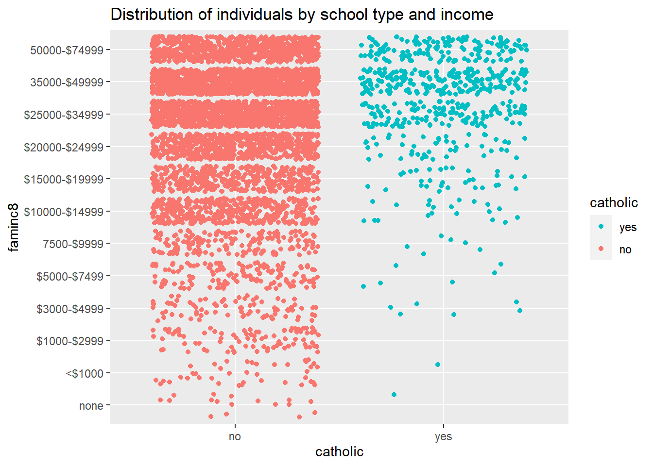

Generating Variable Categories

The book examples uses generated variables faminc8, which uses the actual mid-values of each income range, scaled.

nels88 <- nels88 %>%
  mutate(inc8 = dplyr::recode(faminc8,
    "1" = 0,
    "2"=.5,
    "3"=2,
    "4"=4,
    "5"=6.25,
    "6"=8.75,
    "7"=12.5,
    "8"=17.5,
    "9"=22.5,
    "10"=30,
    "11"=42.5,
    "12"=62.5
  ))

Determining the Best Model

Before generating propensity scores, it is important to determine the best model that predicts group membership through an iterative process.

# this functions adds chi-square to model summary outputs
glance_custom.glm <- function(x) {
    lrchi2 <- lmtest::lrtest(x)[2,4]
    lrchi2out <- tibble::tibble(`LR Chi-Square:` = lrchi2)
    return(lrchi2out)
}

nels88_modela <- glm(catholic ~ (inc8*math8),
                     data=nels88, family="binomial")

nels88_modelb <- glm(catholic ~ I(inc8^2) + (inc8*math8),
                     data=nels88, family="binomial")

nels88_modelc <- glm(catholic ~ I(inc8^2) + (inc8*math8) + fhowfar + mhowfar + fight8 + nohw8 + disrupt8 + riskdrop8,
                     data=nels88, family="binomial")

msummary(list(
  "Model A" = nels88_modela, 
  "Model B" = nels88_modelb,
  "Model c" = nels88_modelc)) %>%
  apa_msummary("Parameter estimates and approximate p-values for a set of fitted logistic regression models in which attendance at a public or a Catholic high school (CATHOLIC) has been regressed on hypothesized selection predictors (INC8 and MATH8) that describe the base-year annual family income and student mathematics achievement (n = 5,671)")

Parameter estimates and approximate p-values for a set of fitted logistic regression models in which attendance at a public or a Catholic high school (CATHOLIC) has been regressed on hypothesized selection predictors (INC8 and MATH8) that describe the base-year annual family income and student mathematics achievement (n = 5,671)

	Model A	Model B	Model c
(Intercept)	-5.209	-5.362	-4.982
	(0.586)	(0.619)	(0.703)
inc8	0.062	0.087	0.054
	(0.014)	(0.017)	(0.019)
inc8:math8	-0.001	-0.001	-0.000
	(0.000)	(0.000)	(0.000)
math8	0.043	0.036	0.022
	(0.011)	(0.012)	(0.012)
I(inc8^2)		-0.000	-0.000
		(0.000)	(0.000)
disrupt8			0.693
			(0.386)
fhowfar			0.196
			(0.087)
fight8			-0.474
			(0.325)
mhowfar			0.026
			(0.087)
nohw8			-0.688
			(0.176)
riskdrop8			-0.303
			(0.084)
Num.Obs.	5671	5671	5671
AIC	3683.2	3677.1	3630.3
BIC	3709.8	3710.3	3703.3
Log.Lik.	-1837.592	-1833.541	-1804.125
LR Chi-Square:	120.129	128.231	187.063

Interpretations

Model C was determined to be the best based on having smaller model fit statistics AIC/BIC. Also, since Model B is nested within Model C, we can perform a Likelihood-Ratio Chi-squared test between the model deviances (i.e., $-2\times LL$): $(-2 \times -1833.541) - (-2\times -1804.125) = 58.8$, which is distibuted as a Chi-squared with degrees of freedom equal the difference in the number of paramters between models (10-4 = 6): $\chi^2$(6)=58.8, p < .001.

Note: a polynomial term ($inc8^2$) to account for a non-linear relationship between catholic and inc8. See Box-Tidwell (i.e., adding interactions between the continuous variables and its natural log, if it’s significant, it suggest non-linearity) and link tests (i.e., this uses the predicted values and square of predicted values to test whether the model is properly specified, the squared term should not be statistically significant) for logistic regression.

Examining the Region of Common Support

These graphics show the overlap of the propensity scores of the two groups, suggesting they share a lot of common support on the covariates in the model. Common support indicates the regions of stratification share enough members of the treatment and control groups.

# Create Propensity Scores
nels88_propscore <- data.frame(pr_score = predict(nels88_modelc,
                                  type="response")) %>%
  add_column(nels88_modelc$data)

nels88_propscore %>%
  mutate(catholic = ifelse(catholic == 1, "Catholic", "Public")) %>%
  ggplot()+
  geom_histogram(aes(x=pr_score, y=..density..,), color="white", bins=30)+
  geom_density(aes(x=pr_score))+
  facet_wrap(~catholic, ncol=1)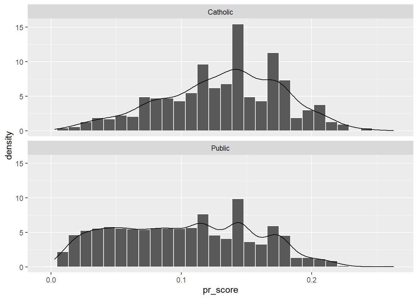

nels88_propscore %>%
  mutate(catholic = ifelse(catholic == 1, "Catholic", "Public")) %>%
  ggplot()+
  geom_histogram(aes(x=pr_score, y=..density.., fill=catholic), color="white", bins=30, position="identity", alpha=.3)+
  geom_density(aes(x=pr_score, color=catholic))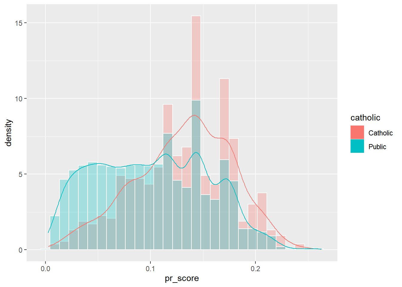

Stratifying on the Propensities

Stratification into 5 blocks based on quintiles

# making quintiles
nels88_5blocks <- nels88_propscore %>%
  mutate(blocks = ntile(pr_score, 5),
         catholic = factor(catholic, labels = c(
           "Catholic", "Public"
         ))) %>%
  group_by(blocks)

Checking balance on the propensities

do(nels88_5blocks, tidy(t.test(.$pr_score ~ .$catholic,
                 alternative = "greater",
                 paired = FALSE,
                 var.equal = TRUE,
                 conf.level = 0.95
                 ))) %>%
  select(blocks, p.value) %>%
  ungroup() %>%
  apa("Testing balance of blocks based on quntiles")

Testing balance of blocks based on quntiles

blocks	p.value
1	0.9846739
2	0.9996522
3	0.9851109
4	0.7720567
5	0.9508310

Interpretation

The table above shows t-tests per block between propensity scores and treatment groups. Using a one-sided test where the expectation is a greater score, none of the differences are significant. This suggests balance.

Note: if you choose “less”, you will get different results becuase it is the lower side of the one-sided t-test. You’d be testing whether the expectation is a lower score. You may also want to check individual covariate balance, as below.

Stratification into 5 blocks based on cut scores

The following stratification comes from p. 320

nels88_5blocks_2 <- nels88_propscore %>%
  mutate(blocks = case_when(
    pr_score < .05 ~ 1,
    pr_score = .05 & pr_score <.1 ~2,
    pr_score =.1 & pr_score <.15 ~ 3,
    pr_score = .15 & pr_score < .2 ~ 4,
    pr_score = .2 & pr_score < .3 ~ 5
  ),
  catholic = factor(catholic, labels = c(
           "Public", "Catholic"
         ))) %>%
  group_by(blocks)

do(nels88_5blocks_2, tidy(t.test(.$pr_score ~ .$catholic,
                 alternative = "greater",
                 paired = FALSE,
                 var.equal = TRUE,
                 conf.level = 0.95
                 ))) %>%
  select(blocks, p.value) %>%
  ungroup() %>%
  apa("Testing balance of blocks based on the book's example")

Testing balance of blocks based on the book's example

blocks	p.value
1	0.9788125
2	0.9884155
3	0.9776620
4	0.9145168
5	0.2712632

Estimate the ATE and ATT of Stratified Propensity Scores

# Summarize Block
nels88_5blocks_sum <- nels88_5blocks_2 %>%
  group_by(blocks, catholic) %>%
  summarize(n = n(),
    pr_score = mean(pr_score),
            income_mean=mean(inc8),
            mathmean = mean(math8),
            math_achievment = mean(math12)) %>%
  pivot_wider(names_from=catholic, values_from = c(n, pr_score, income_mean, mathmean, math_achievment)) %>%
  mutate(diff = math_achievment_Catholic - math_achievment_Public,
         n = n_Catholic + n_Public,
         mutate(across(where(is.numeric), round, 3))) %>%
  ungroup()

## `summarise()` regrouping output by 'blocks' (override with `.groups` argument)

apa(nels88_5blocks_sum, "Five propensity-score blocks, based on predicted values from final Model C (which contains selected covariates in addition to those included in Model B). Within-block sample statistics include: (a) frequencies, (b) average propensity scores, and (c) average twelfth grade mathematics achievement by type of high school, and their difference (n = 5,671)")

Five propensity-score blocks, based on predicted values from final Model C (which contains selected covariates in addition to those included in Model B). Within-block sample statistics include: (a) frequencies, (b) average propensity scores, and (c) average twelfth grade mathematics achievement by type of high school, and their difference (n = 5,671)

blocks	n_Public	n_Catholic	pr_score_Public	pr_score_Catholic	income_mean_Public	income_mean_Catholic	mathmean_Public	mathmean_Catholic	math_achievment_Public	math_achievment_Catholic	diff	n
1	1089	34	0.030	0.035	13.316	13.169	44.542	46.039	43.664	46.014	2.350	1123
2	1431	110	0.075	0.078	27.017	26.675	49.412	49.956	48.853	51.002	2.149	1541
3	1599	253	0.127	0.129	35.930	37.362	53.891	53.971	53.623	55.383	1.760	1852
4	829	160	0.172	0.173	52.289	52.891	58.048	57.814	56.869	57.346	0.477	989
5	131	35	0.213	0.212	59.752	60.214	51.304	51.475	52.506	55.013	2.507	166

#Weighted Average Treatment Effect
nels88_5blocks_sum %>%
  mutate(weighted = diff * n) %>%
  pull(weighted) %>%
  sum()/sum(nels88_5blocks_sum$n)

## [1] 1.780655

#Weighted Average Treatment on the Treated Effect
nels88_5blocks_sum %>%
  mutate(weighted = diff * n_Catholic) %>%
  pull(weighted) %>%
  sum()/sum(nels88_5blocks_sum$n_Catholic)

## [1] 1.563573

Using MatchIt

Method from http://www.practicalpropensityscore.com/matching.html

library(MatchIt)

set.seed(2020)

#generate propensity scores using Model C
nels88_ps <- matchit(catholic ~ I(inc8^2) + (inc8*math8) + fhowfar + mhowfar + fight8 + nohw8 + disrupt8 + riskdrop8,
                         data=nels88,
                         method="nearest", #nearest neighbors
                         replace=T, #with replacement
                        ratio=1) #one to one matching - each treated with one control
                    
                    #A user may want to consider adding a caliper option to only select cases within a certain range, caliper = .2

Diagnose Covariate Balance

nels88_ps_sum <- summary(nels88_ps)

#raw
#summary(abs(nels88_ps_sum$sum.matched$`Mean Diff`))

This table shows the maximum standardized mean difference in propensity scores ? between groups.

summary(abs(summary(nels88_ps, standardize = T)$sum.matched$`Std. Mean Diff`))

##     Min.  1st Qu.   Median     Mean  3rd Qu.     Max. 
## 0.000000 0.004342 0.020411 0.021566 0.036718 0.051833

The results show Small differences between groups on the covariates. (Max = .05).

table(abs(summary(nels88_ps, standardize = T)$sum.matched$"Std. Mean Diff.") > .1) #Table says Max = .05, but this function says there are 11 cases with Std.Mean.Diff > .1

## 
## FALSE 
##    11

This table shows that only there are no differences greater than .1 (FALSE 11)

Estimate Treatment Effects

#obtain matched data
matched_data <- match.data(nels88_ps)

# use weights to estimate ATT
library(survey)
design.nels88 <- svydesign(ids=~1, weights=~weights,
                                   data=matched_data)
#estimate the ATT 
model.nels88 <- svyglm(math12~catholic + I(inc8^2) + (inc8*math8) + fhowfar + mhowfar + fight8 + nohw8 + disrupt8 + riskdrop8, design.nels88, family=gaussian())

summary(model.nels88)

## 
## Call:
## svyglm(formula = math12 ~ catholic + I(inc8^2) + (inc8 * math8) + 
##     fhowfar + mhowfar + fight8 + nohw8 + disrupt8 + riskdrop8, 
##     design = design.nels88, family = gaussian())
## 
## Survey design:
## svydesign(ids = ~1, weights = ~weights, data = matched_data)
## 
## Coefficients:
##               Estimate Std. Error t value Pr(>|t|)    
## (Intercept)  5.2344350  2.5150613   2.081 0.037641 *  
## catholic     1.2250485  0.3128480   3.916 9.56e-05 ***
## I(inc8^2)   -0.0013863  0.0006069  -2.284 0.022542 *  
## inc8         0.2410835  0.0681540   3.537 0.000421 ***
## math8        0.8123924  0.0426961  19.027  < 2e-16 ***
## fhowfar     -0.0421049  0.4213556  -0.100 0.920420    
## mhowfar      0.4604611  0.4064090   1.133 0.257459    
## fight8       0.3835736  1.5872490   0.242 0.809089    
## nohw8       -1.9228815  0.6605490  -2.911 0.003674 ** 
## disrupt8    -0.3809514  1.7834881  -0.214 0.830899    
## riskdrop8   -0.1132044  0.3294263  -0.344 0.731181    
## inc8:math8  -0.0020930  0.0010155  -2.061 0.039521 *  
## ---
## Signif. codes:  0 '***' 0.001 '**' 0.01 '*' 0.05 '.' 0.1 ' ' 1
## 
## (Dispersion parameter for gaussian family taken to be 25.95404)
## 
## Number of Fisher Scoring iterations: 2

Because of unmatched controls (4,546; see summary(nels88_ps)), we can typically only estimate the ATT since we don’t typically include the entire sample. Weighting by the inverse of the propensity score then running the analysis is one way to get the ATE. You can also get ATE from stratification.

Another MatchIt Method

From Propensity Scores: A Practical Introduction Using R

Visualize Propensity Scores

plot(nels88_ps, type ="jitter")

## [1] "To identify the units, use first mouse button; to stop, use second."

## integer(0)

Prepare Matched Data

# save matched data
matches <- data.frame(nels88_ps$match.matrix)

# find the  matches
group1 <- match(row.names(matches), row.names(matched_data))
group2 <- match(matches$X1, row.names(matched_data))

# extract outcome values for matches
treatment <- matched_data$math12[group1]
control <- matched_data$math12[group2]

# create matched data set
outcomes <- cbind(matches, treatment, control)

# t-test
t.test(outcomes$treatment, outcomes$control, paired = T) %>% 
  tidy() %>%
  select(estimate:p.value, method, alternative) %>%
  apa("Outcome Analysis")

Outcome Analysis

estimate	statistic	p.value	method	alternative
0.939831	2.22596	0.02639323	Paired t-test	two.sided

.93 is the ATT. It is lower than what’s found in the Methods Matter, but it also uses a slightly different method. One thing we’d want to do is assess the robustness of these results by altering parameters of the matching algorithm (e.g., adding a caliper, altering the values of the caliper .2 to .15, matching with and without replacement, ratio matching 1:5) or by choosing a different matching algorithm (e.g., optimal matching, full matching). These type of tests help demonstrate that results do not depend on the particular matching method chosen.

Stratification with MatchIt

Based on Practical Propensity Score Methods Using R (Leite, 2019)

formula <- formula("catholic ~ I(inc8^2) + (inc8*math8) + fhowfar + mhowfar + fight8 + nohw8 + disrupt8 + riskdrop8")

# make the subclasses
nels_stratified <- matchit(formula, #formula
                          distance=nels88_propscore$pr_score, #propensity scores
                          data = nels88_propscore, #data
                          method = "subclass", #statifying method
                          sub.by = "treat",
                          subclass=5) # quintiles

# get the matched data
data.stratification <- match.data(nels_stratified) %>%
  mutate(catholic = factor(catholic, labels=c("Public", "Catholic")))
  
#preview
data.stratification %>%
  janitor::tabyl(catholic, subclass)

##  catholic    1    2   3   4   5
##    Public 2198 1016 702 616 547
##  Catholic  119  118 118 118 119

Covariate Balance Evaluation

# obtain standardize mean differences
balance.stratification <- summary(nels_stratified, standardize=T)

# the following extracts only the standardized mean differences for all strata
balance.stratification$q.table[,3,] %>%
  as.data.frame() %>%
  pivot_longer("Subclass 1":"Subclass 5", names_to = "strata", values_to="mean_diff") %>%
  group_by(strata) %>%
  summarize(min = min(mean_diff),
            mean = mean(mean_diff),
            max = max(mean_diff))

## # A tibble: 5 x 4
##   strata         min     mean    max
##   <chr>        <dbl>    <dbl>  <dbl>
## 1 Subclass 1 -0.565   0.00616 0.271 
## 2 Subclass 2 -0.0656  0.0478  0.144 
## 3 Subclass 3 -0.0764  0.00674 0.0739
## 4 Subclass 4 -0.102  -0.00880 0.0317
## 5 Subclass 5 -0.0108  0.0328  0.0837

Two stratas have greater than .1 and 1 has greater than .25. This is OK, but not great.

Obtaining ATE and ATE Estimates

design <- svydesign(ids=~0, 
                    weights=~weights,
                    data=data.stratification)

# Robust SE through bootstrapping
# Good for when not known or easy formula

set.seed(2020)

surveyDesignBoot <- as.svrepdesign(design, type=c("bootstrap"),replicates=1000)

#obtain means and standard errors by stratum and treatment group combinations

subclassMeans <- svyby(formula=~math12, 
                        by=~catholic+subclass,
                        design=surveyDesignBoot,
                        FUN=svymean,
                       covmat=TRUE)

# get weights for estimation

weights <- data.stratification %>%
  janitor::tabyl(catholic, subclass) %>%
  pivot_longer(`1`:`5`, names_to = "strat", values_to = "n") %>%
  pivot_wider(names_from = catholic, values_from=n) %>%
  mutate(strat_sum = Public + Catholic,
         total_treated = sum(Catholic),
         total_n = sum(strat_sum),
         ATE_wk = strat_sum/total_n,
         ATT_wk = Catholic/total_treated)

# estimation via linear/nonlinear contrasts
pooledEffects <- svycontrast(subclassMeans, list(
    ATE=c(rbind(-weights$ATE_wk, weights$ATE_wk)),
    ATT=c(rbind(-weights$ATT_wk, weights$ATT_wk))))

pooledEffects

##     contrast    SE
## ATE   2.1079 0.404
## ATT   1.6107 0.364