Chapter 3 May 30–Jun 4: Synchronous seminar
In this week of HE930, we will meet synchronously on Zoom to examine the predictive analytics process, discuss the ethics of using predictive analytics in HPEd, and apply predictive analytics together to a dataset.
Note that there is no assignment to complete and turn in this week. The only required work this week is to attend the synchronous seminar sessions on Zoom. Please try your best to attend these sessions. If you cannot attend, we will arrange for make-up activities for you to complete.
MOST IMPORTANTLY, please complete the following preparation before you attend the synchronous seminar sessions.
3.1 Preparation for synchronous seminar
Please watch the following two videos, which we will discuss in our synchronous seminar:
- “Predictive Analytics in Education: An introductory example”. https://youtu.be/wGE7C5w6hb4. Available on YouTube and also embedded below.
The slides for the video above are available at https://rpubs.com/anshulkumar/ClassificationExample2020.
The Social Dilemma on Netflix. This link might take you there: https://www.netflix.com/title/81254224. If you do not have access to this on your own, inform the course instructors and we will arrange for you to watch.
Finally, in addition to watching the two videos above, please review all Week 1 readings, if you have not done so already.
Once you complete the items above, you do not need to do anything else other than attending the scheduled synchronous sessions on Zoom.
3.2 Seminar details
Schedule as of May 29 2023:
The Analytics Process. Thursday June 1 2023, 11 a.m. – 1 p.m. Boston time. To prepare for this session, please review all Week 1 readings and watch this 26-minute video: https://youtu.be/wGE7C5w6hb4.
Machine Learning in R. Part 1: Thursday June 1 2023, 1–2 p.m. Boston time; Part 2: Friday June 2 2023, 1–2 p.m. Boston time. During this session, we will do a machine learning tutorial in R and RStudio on our computers. Please be prepared to run RStudio on your computer and share your screen. No other preparation for this session is needed.
The Social Dilemma and Ethical Concerns of ML. Friday June 2 2023, 11 a.m. – 1 p.m. Boston time. To prepare for this session, please watch The Social Dilemma on Netflix, which you can access at https://www.netflix.com/title/81254224.
You should have received calendar invitations to your email address for the sessions above. We will see who all is able to attend the sessions above. Then, for those who are not able to attend, we will schedule additional sessions in which the topics above will be repeated.
3.3 Session 1: The Analytics Process
3.3.1 Goal 1: Discuss the PA process and its applications
Reminder:
- PA = predictive analytics
- ML = machine learning
- AI = artificial intelligence
This discussion will primarily be driven by questions and topics raised by students during the sessions itself. The items listed below are meant to supplement our discussion.
3.3.2 Questions & topics from weeks 1 & 2 discussion posts
3.3.2.1 What is PA/ML and how do we conduct it?
Item 1: “I would like to learn more about the early alert systems these schools were able to use and how to build something like that.” (DR)
Item 2: “Recent work on learning analytics based on students’ online engagement highlights the importance of students’ internal conditions as well as external factors as indicators of their performance.” (SA)
3.3.2.2 Using PA/ML in HPEd
Item 3: “The article makes use of a single course in a single medical university and hence the findings may not be generalizable.” (SA)
Item 4: “how are predictive analytics being used at MGIHP and in the PhD? I am also curious about Nicole’s and Anshul’s thoughts about the ethicality, bias and the role disclosure to learners when predictive analytics are being used.” (FS)
3.3.2.3 Ethics of PA/ML
Item 5: “I would have liked more transparency about how and which data were used from assignments/discussions, however: ‘The process of establishing features from raw data in the database was realized automatically via the help of an in-house developed tool.’ [(Akçapınar 2019)] That said, there is a good Appendix (Table 14) that spells out which data were used.” (DR)
Item 6: “several of the metrics are related to number or amount of time spent visiting a particular part of the course site. As we all know, it is easy to access a page and then minimize it without interacting with the content. If the numbers are very high in this area, it may skew results.” (DR)
Item 7: “As described in the beginning of the Ekowo and Palmer article, this type of information can be used for less than altruistic purposes- to deter students who are unlikely to pass and therefore will reflect poorly on the metrics published about the university.” (DR)
Item 8: Possible risks of using PA/ML in education…
- “Data selection bias - unintentional stereotyping” (DT)
- “Breach of confidentiality” / “Misuse of student information” (DT)
- “The use of analytic process to predict college academic success has huge potentials for discrimination, labeling and stigma, and if not implemented correctly are potential sources of ethical and legal issues in higher education.” (RB)
- “May be used to perpetuate bias and/or structural racism in academia.” (FS)
- “There is also the issue of mistrust and potential lack of transparency regarding how the data will be stored, shared, and used outside of the stated intent.” (FS)
Item 9: “As we know, there are different types of learners. Some students would thrive using the online platform methods of learning. Some students may not. It does not mean they are less intelligent. It simply means that those individual students retain and utilize knowledge differently. So, I do worry about creating a system where the number of logins, the time spent, number of contents created, etc. are used as markers for student success. It gives an arbitrary meaning to the term ‘success,’ if we are only defining success by their performance on the online platform and the final course grade.” (MM)
Item 10: “With course signals, leaners are assigned a color based on their risk level, this could lead to labeling and foster a class system within the learning community.” (JM)
Item 11: “I find this topic to be fascinating as I reflect back on my academic experience in undergraduate studies. The common sentiment to someone heading into college can be, ‘You need to be accountable for your work and your time, no one is going to be checking in to see if you’re handing in your work or not.’ This can be true, however, to note how universities do care for the wellbeing of their students (and not just for performative reasons) is an essential piece for not only students in the classroom, but also how they then take what they learn and bring it into their careers.” (ED)
Item 12: “The vulnerable period of adjustment, especially for certain groups with most factors for academic failure is a critical period for colleges/universities for identification and provision of academic support such as targeted advising and adaptive learning.” (RB)
3.3.2.4 Disseminating/communicating results
Item 13: JM pointed out that many forms of intervention were used in the Arnold and Pistilli study, including traffic signal indicator in LMS, emails, text messages, referrals to advisors or resource centers, face to face meetings with instructor. (JM)
Item 14: “Please share why these 3 articles were selected vs. others?” (FS)
3.3.3 Discussion questions from PA video/slides
How can predictive/learning analytics help you in your own work as an educator or at your organization/institution? What predictions would be useful for you to make?
How can you leverage data that your institution already collects (or that it is well-positioned to collect) using predictive analytic methods?
What would be the benefits and detriments of incorporating predictive analytics into your institution’s practices and processes?
Could predictive analysis complement any already-ongoing initiatives at your institution?
What would the ethical implications be of using predictive analytics at your institution? Would it cause unfair discrimination against particular learners? Would it help level the playing field for all learners?
3.4 Session 2: Machine Learning in R
During this session, we will work together to complete and discuss the machine learning tutorial below.
3.4.1 Goals
Practice using decision tree and logistic regression models to predict which students are going to pass or fail, using the
student-por.csvdata.Fine-tune predictive models.
Compare the results of different predictive models and choose the best one.
Brainstorm about how the predictions would be used in an educational setting.
3.4.2 Important reminders
Anywhere you see the word
MODIFYis one place where you might consider making changes to the code.If you are not certain about any interpretations of results—especially confusion matrices, accuracy, sensitivity, and specificity—stop and ask an instructor for assistance.
For most of this tutorial, you will run the code below in an R script or R markdown file in RStudio on your own computer. You will also make minor modifications to this code.
3.4.3 Load relevant packages
Step 1: Load packages
if (!require(PerformanceAnalytics)) install.packages('PerformanceAnalytics') ## Warning: package 'xts' was built under R
## version 4.2.3## Warning: package 'zoo' was built under R
## version 4.2.3if (!require(rpart)) install.packages('rpart')
if (!require(rpart.plot)) install.packages('rpart.plot')
if (!require(car)) install.packages('car') ## Warning: package 'car' was built under R
## version 4.2.3if (!require(rattle)) install.packages('rattle') ## Warning: package 'tibble' was built under
## R version 4.2.3library(PerformanceAnalytics)
library(rpart)
library(rpart.plot)
library(car)
library(rattle)3.4.4 Import and describe data
We will use the student-por.csv data.
Step 2: Import data
d <- read.csv("student-por.csv")The best place to download this data is from D2L.
Data source and details:
P. Cortez and A. Silva. Using Data Mining to Predict Secondary School Student Performance. In A. Brito and J. Teixeira Eds., Proceedings of 5th FUture BUsiness TEChnology Conference (FUBUTEC 2008) pp. 5-12, Porto, Portugal, April, 2008, EUROSIS, ISBN 978-9077381-39-7. Available at https://archive.ics.uci.edu/ml/datasets/Student+Performance.
Alternate source: https://www.kaggle.com/larsen0966/student-performance-data-set
If the code above does not work to load the data, you can try this code instead:
d <- read.csv(file = "student-por.csv", sep = ";")Step 3: List variables
names(d)## [1] "school" "sex"
## [3] "age" "address"
## [5] "famsize" "Pstatus"
## [7] "Medu" "Fedu"
## [9] "Mjob" "Fjob"
## [11] "reason" "guardian"
## [13] "traveltime" "studytime"
## [15] "failures" "schoolsup"
## [17] "famsup" "paid"
## [19] "activities" "nursery"
## [21] "higher" "internet"
## [23] "romantic" "famrel"
## [25] "freetime" "goout"
## [27] "Dalc" "Walc"
## [29] "health" "absences"
## [31] "G1" "G2"
## [33] "G3"Description of dataset and all variables: https://archive.ics.uci.edu/ml/datasets/Student+Performance.
All variables in formula (for easy copying and pasting):
(b <- paste(names(d), collapse="+"))## [1] "school+sex+age+address+famsize+Pstatus+Medu+Fedu+Mjob+Fjob+reason+guardian+traveltime+studytime+failures+schoolsup+famsup+paid+activities+nursery+higher+internet+romantic+famrel+freetime+goout+Dalc+Walc+health+absences+G1+G2+G3"Step 4: Calculate number of observations
nrow(d)## [1] 649Step 5: Generate binary version of dependent variable, G3 (final grade, 0 to 20).
d$passed <- ifelse(d$G3 > 9.99, 1, 0)We’re assuming that a score of over 9.99 is a passing score, and below that is failing.
Step 6: Descriptive statistics for G3 continuous numeric variable.
summary(d$G3)## Min. 1st Qu. Median Mean 3rd Qu.
## 0.00 10.00 12.00 11.91 14.00
## Max.
## 19.00sd(d$G3)## [1] 3.230656Step 7: Who all passed and failed, binary qualitative categorical variable.
with(d, table(passed, useNA = "always"))## passed
## 0 1 <NA>
## 100 549 0Step 8: Histogram
hist(as.numeric(d$G3))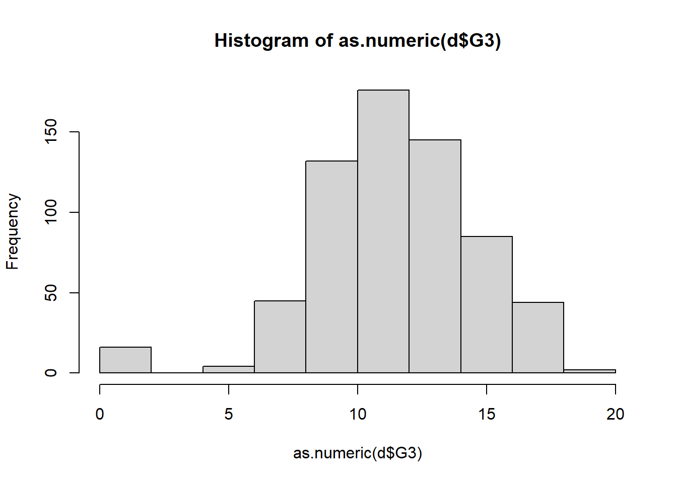
Step 9: Scatterplots
plot(d$G1 , d$G3) # MODIFY which variables you plot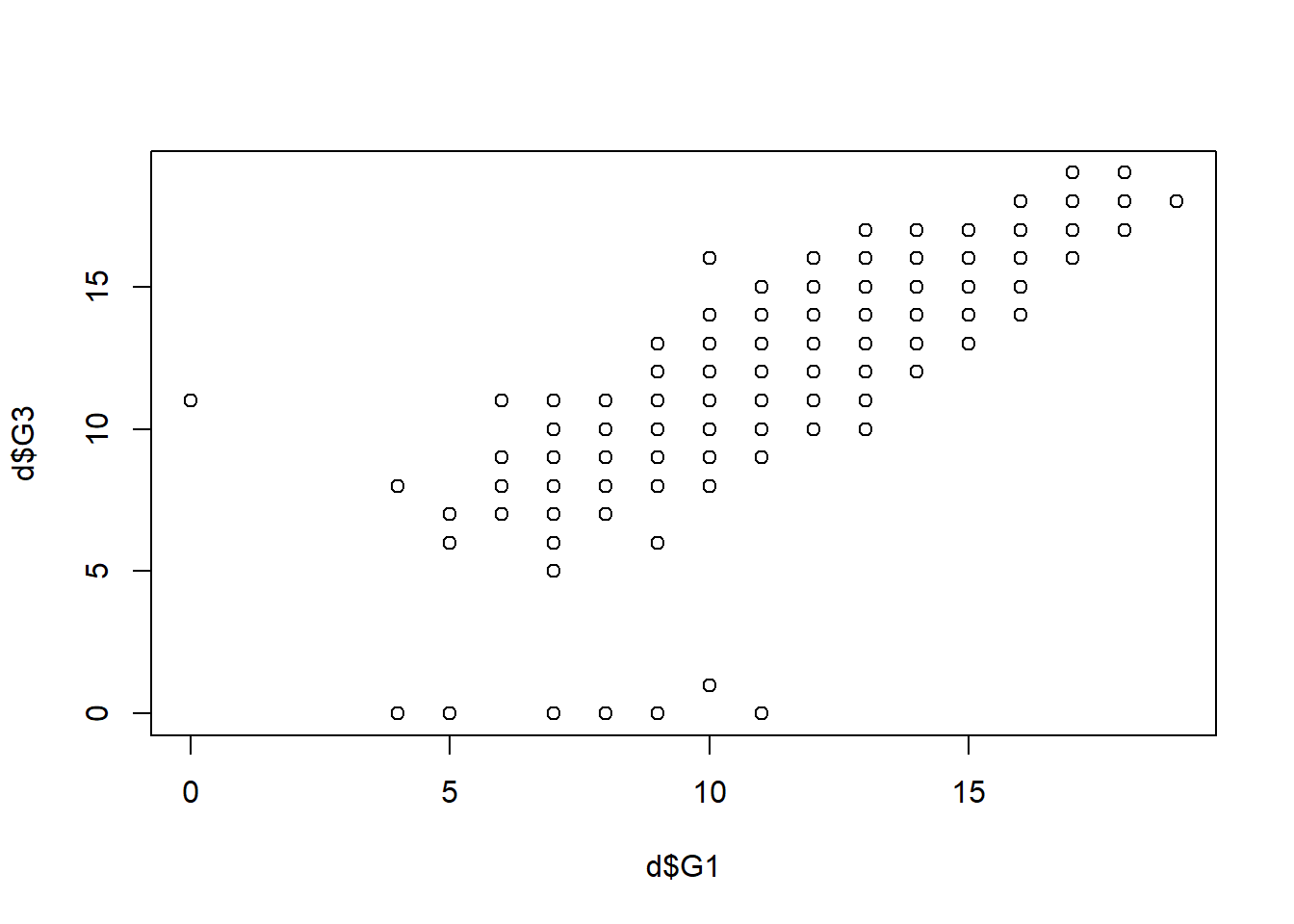
plot(d$health, d$G3)
Step 10: Selected correlations (optional)
chart.Correlation(d[c("G3","G1","Medu","failures")], histogram=TRUE, pch=19) ## Warning in par(usr): argument 1 does not
## name a graphical parameter
## Warning in par(usr): argument 1 does not
## name a graphical parameter
## Warning in par(usr): argument 1 does not
## name a graphical parameter
## Warning in par(usr): argument 1 does not
## name a graphical parameter
## Warning in par(usr): argument 1 does not
## name a graphical parameter
## Warning in par(usr): argument 1 does not
## name a graphical parameter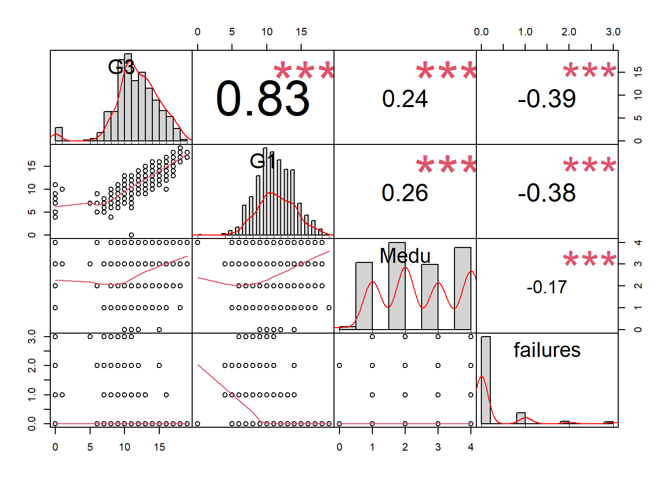
3.4.5 Divide training and testing data
Step 11: Divide data
trainingRowIndex <- sample(1:nrow(d), 0.75*nrow(d))  # row indices for training data
dtrain <- d[trainingRowIndex, ]  # model training data
dtest <- d[-trainingRowIndex, ] # test data3.4.6 Decision tree model – regression tree
Activity summary:
- Goal: predict continuous outcome
G3, using a regression tree. - Start by using all variables to make decision tree. Check predictive capability.
- Remove variables to make predictions with less information.
- Modify cutoff thresholds and see how confusion matrix changes.
- Anywhere you see the word
MODIFYis one place where you might consider making changes to the code. - Figure out which students to remediate.
3.4.6.1 Train and inspect model
Step 14: Train a decision tree model
tree1 <- rpart(G3 ~ school+sex+age+address+famsize+Pstatus+Medu+Fedu+Mjob+Fjob+reason+guardian+traveltime+studytime+failures+schoolsup+famsup+paid+activities+nursery+higher+internet+romantic+famrel+freetime+goout+Dalc+Walc+health+absences+G1+G2, data=dtrain, method = 'anova')
# MODIFY. Complete the next step (visualize the tree) and
# then come back to this and run the model without G1 and
# G2. Then try other combinations.

summary(tree1)
## Call:
## rpart(formula = G3 ~ school + sex + age + address + famsize +
## Pstatus + Medu + Fedu + Mjob + Fjob + reason + guardian +
## traveltime + studytime + failures + schoolsup + famsup +
## paid + activities + nursery + higher + internet + romantic +
## famrel + freetime + goout + Dalc + Walc + health + absences +
## G1 + G2, data = dtrain, method = "anova")
## n= 486
##
## CP nsplit rel error xerror
## 1 0.51625308 0 1.0000000 1.0052137
## 2 0.14623666 1 0.4837469 0.4893097
## 3 0.09730706 2 0.3375103 0.3683695
## 4 0.04549495 3 0.2402032 0.2704503
## 5 0.03097591 4 0.1947083 0.2325672
## 6 0.01853902 5 0.1637323 0.2048112
## 7 0.01000000 6 0.1451933 0.1861552
## xstd
## 1 0.09980294
## 2 0.06358710
## 3 0.04290278
## 4 0.04178559
## 5 0.03703264
## 6 0.03574689
## 7 0.03566205
##
## Variable importance
## G2 G1 failures
## 42 24 7
## school Medu Dalc
## 7 7 5
## absences famrel famsize
## 2 1 1
## famsup traveltime Mjob
## 1 1 1
## health
## 1
##
## Node number 1: 486 observations, complexity param=0.5162531
## mean=11.93004, MSE=10.28729
## left son=2 (243 obs) right son=3 (243 obs)
## Primary splits:
## G2 < 11.5 to the left, improve=0.5162531, (0 missing)
## G1 < 11.5 to the left, improve=0.4413648, (0 missing)
## failures < 0.5 to the right, improve=0.2305066, (0 missing)
## higher splits as LR, improve=0.1141877, (0 missing)
## school splits as RL, improve=0.0809182, (0 missing)
## Surrogate splits:
## G1 < 11.5 to the left, agree=0.877, adj=0.753, (0 split)
## school splits as RL, agree=0.634, adj=0.267, (0 split)
## failures < 0.5 to the right, agree=0.632, adj=0.263, (0 split)
## Medu < 3.5 to the left, agree=0.613, adj=0.226, (0 split)
## Dalc < 1.5 to the right, agree=0.603, adj=0.206, (0 split)
##
## Node number 2: 243 observations, complexity param=0.1462367
## mean=9.625514, MSE=6.711612
## left son=4 (23 obs) right son=5 (220 obs)
## Primary splits:
## G2 < 7.5 to the left, improve=0.44829120, (0 missing)
## G1 < 8.5 to the left, improve=0.24780240, (0 missing)
## failures < 0.5 to the right, improve=0.14649750, (0 missing)
## school splits as RL, improve=0.05266388, (0 missing)
## absences < 0.5 to the left, improve=0.04923970, (0 missing)
##
## Node number 3: 243 observations, complexity param=0.09730706
## mean=14.23457, MSE=3.241274
## left son=6 (130 obs) right son=7 (113 obs)
## Primary splits:
## G2 < 13.5 to the left, improve=0.61767410, (0 missing)
## G1 < 14.5 to the left, improve=0.43851760, (0 missing)
## schoolsup splits as RL, improve=0.06724359, (0 missing)
## age < 16.5 to the left, improve=0.05527754, (0 missing)
## Mjob splits as LRLLR, improve=0.05421553, (0 missing)
## Surrogate splits:
## G1 < 13.5 to the left, agree=0.827, adj=0.628, (0 split)
## Mjob splits as LRLLR, agree=0.609, adj=0.159, (0 split)
## Medu < 3.5 to the left, agree=0.601, adj=0.142, (0 split)
## health < 2.5 to the right, agree=0.584, adj=0.106, (0 split)
## age < 17.5 to the left, agree=0.576, adj=0.088, (0 split)
##
## Node number 4: 23 observations, complexity param=0.04549495
## mean=4.26087, MSE=14.19282
## left son=8 (12 obs) right son=9 (11 obs)
## Primary splits:
## absences < 1 to the left, improve=0.6967931, (0 missing)
## G2 < 5.5 to the left, improve=0.3995738, (0 missing)
## famsup splits as LR, improve=0.3048272, (0 missing)
## age < 17.5 to the right, improve=0.2083941, (0 missing)
## internet splits as LR, improve=0.1920796, (0 missing)
## Surrogate splits:
## G2 < 2.5 to the left, agree=0.739, adj=0.455, (0 split)
## famsize splits as LR, agree=0.696, adj=0.364, (0 split)
## traveltime < 1.5 to the right, agree=0.696, adj=0.364, (0 split)
## famsup splits as LR, agree=0.696, adj=0.364, (0 split)
## famrel < 4.5 to the right, agree=0.696, adj=0.364, (0 split)
##
## Node number 5: 220 observations, complexity param=0.03097591
## mean=10.18636, MSE=2.606178
## left son=10 (83 obs) right son=11 (137 obs)
## Primary splits:
## G2 < 9.5 to the left, improve=0.27010620, (0 missing)
## G1 < 9.5 to the left, improve=0.15965460, (0 missing)
## failures < 0.5 to the right, improve=0.12744430, (0 missing)
## higher splits as LR, improve=0.04656336, (0 missing)
## goout < 4.5 to the right, improve=0.03127109, (0 missing)
## Surrogate splits:
## G1 < 8.5 to the left, agree=0.732, adj=0.289, (0 split)
## failures < 0.5 to the right, agree=0.682, adj=0.157, (0 split)
## higher splits as LR, agree=0.645, adj=0.060, (0 split)
## age < 18.5 to the right, agree=0.636, adj=0.036, (0 split)
## famrel < 1.5 to the left, agree=0.632, adj=0.024, (0 split)
##
## Node number 6: 130 observations
## mean=12.91538, MSE=0.862071
##
## Node number 7: 113 observations, complexity param=0.01853902
## mean=15.75221, MSE=1.673115
## left son=14 (69 obs) right son=15 (44 obs)
## Primary splits:
## G2 < 15.5 to the left, improve=0.49025250, (0 missing)
## G1 < 16.5 to the left, improve=0.38024010, (0 missing)
## age < 16.5 to the left, improve=0.04675727, (0 missing)
## Fjob splits as LRLRR, improve=0.04174805, (0 missing)
## Mjob splits as RRLLR, improve=0.03928692, (0 missing)
## Surrogate splits:
## G1 < 15.5 to the left, agree=0.814, adj=0.523, (0 split)
## absences < 0.5 to the right, agree=0.637, adj=0.068, (0 split)
## Fjob splits as LLLLR, agree=0.628, adj=0.045, (0 split)
## Dalc < 2.5 to the left, agree=0.628, adj=0.045, (0 split)
## reason splits as LLRL, agree=0.619, adj=0.023, (0 split)
##
## Node number 8: 12 observations
## mean=1.25, MSE=7.854167
##
## Node number 9: 11 observations
## mean=7.545455, MSE=0.4297521
##
## Node number 10: 83 observations
## mean=9.108434, MSE=2.289447
##
## Node number 11: 137 observations
## mean=10.83942, MSE=1.667643
##
## Node number 14: 69 observations
## mean=15.02899, MSE=0.8977106
##
## Node number 15: 44 observations
## mean=16.88636, MSE=0.78254133.4.6.2 Tree visualization
Step 15: Visualize decision tree model in two ways.
prp(tree1)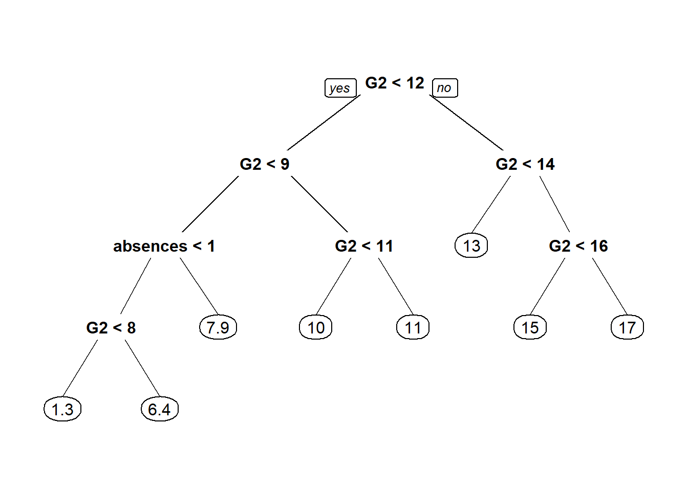
fancyRpartPlot(tree1, caption = "Regression Tree")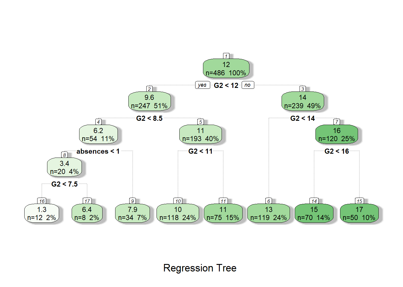
3.4.6.3 Test model
Step 16: Make predictions on testing data, using trained model
dtest$tree1.pred <- predict(tree1, newdata = dtest)Step 17: Visualize predictions
with(dtest, plot(G3,tree1.pred, main="Actual vs Predicted, testing data",xlab = "Actual G3",ylab = "Predicted G3"))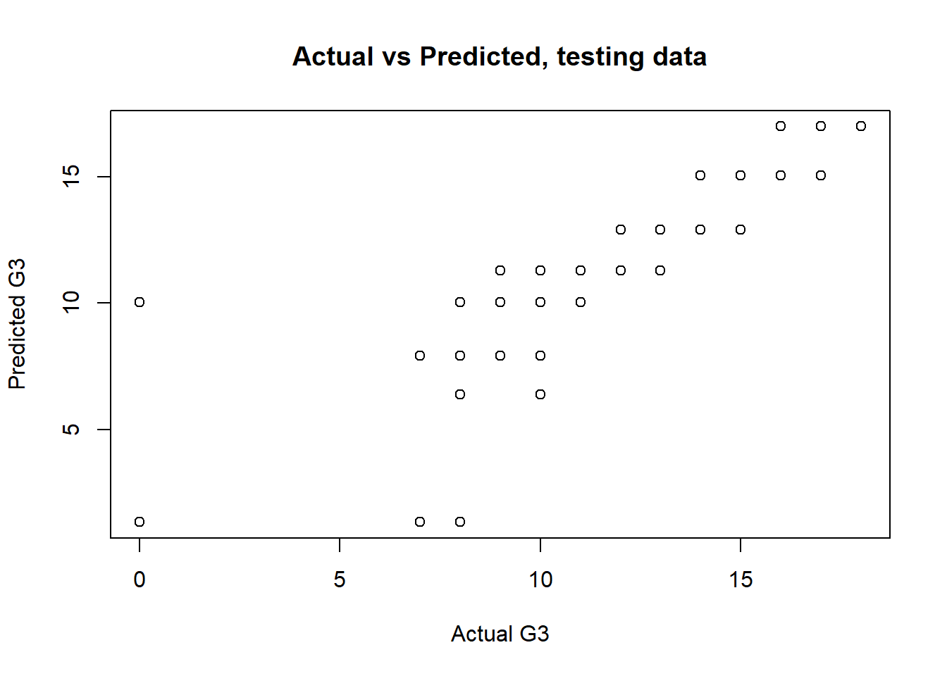
Step 18: Make confusion matrix.
PredictionCutoff <- 9.99 # MODIFY. Compare values in 9-11 range.

dtest$tree1.pred.passed <- ifelse(dtest$tree1.pred > PredictionCutoff, 1, 0)

(cm1 <- with(dtest,table(tree1.pred.passed,passed)))
## passed
## tree1.pred.passed 0 1
## 0 23 16
## 1 1 123Step 19: Calculate accuracy
CorrectPredictions1 <- cm1[1,1] + cm1[2,2]
TotalStudents1 <- nrow(dtest)

(Accuracy1 <- CorrectPredictions1/TotalStudents1)
## [1] 0.8957055Step 20: Sensitivity (proportion of people who actually failed that were correctly predicted to fail).
(Sensitivity1 <- cm1[1,1]/(cm1[1,1]+cm1[2,1]))## [1] 0.9583333Step 21: Specificity (proportion of people who actually passed that were correctly predicted to pass).
(Specificity1 <- cm1[2,2]/(cm1[1,2]+cm1[2,2]))## [1] 0.8848921BE SURE TO DOUBLE-CHECK THE CALCULATIONS ABOVE MANUALLY!
Step 22: It is very important for you, the data analyst, to modify the 9.99 cutoff assigned as PredictionCutoff above to see how you can change the predictions made by the model. Write down what you observe as you change this value and re-run the confusion matrix, accuracy, sensitivity, and specificity code above. What are the implications of your manual modification of this cutoff? Remind your instructors to discuss this, in case they forget!
3.4.7 Decision tree model – classification tree
Activity summary:
- Goal: predict binary outcome
passed, using a classification tree. - Start by using all variables to make decision tree. Check predictive capability.
- Remove variables to make predictions with less information.
- Modify cutoff thresholds and see how confusion matrix changes.
- Anywhere you see the word
MODIFYis one place where you might consider making changes to the code. - Figure out which students to remediate.
3.4.7.1 Train and inspect model
Step 23: Train a decision tree model
tree2 <- rpart(passed ~ school+sex+age+address+famsize+Pstatus+Medu+Fedu+Mjob+Fjob+reason+guardian+traveltime+studytime+failures+schoolsup+famsup+paid+activities+nursery+higher+internet+romantic+famrel+freetime+goout+Dalc+Walc+health+absences+G1+G2, data=dtrain, method = "class")
# MODIFY. Try without G1 and G2. Then try other combinations.

summary(tree2)
## Call:
## rpart(formula = passed ~ school + sex + age + address + famsize +
## Pstatus + Medu + Fedu + Mjob + Fjob + reason + guardian +
## traveltime + studytime + failures + schoolsup + famsup +
## paid + activities + nursery + higher + internet + romantic +
## famrel + freetime + goout + Dalc + Walc + health + absences +
## G1 + G2, data = dtrain, method = "class")
## n= 486
##
## CP nsplit rel error xerror
## 1 0.52631579 0 1.0000000 1.0000000
## 2 0.03289474 1 0.4736842 0.4736842
## 3 0.01973684 3 0.4078947 0.4736842
## 4 0.01000000 5 0.3684211 0.5789474
## xstd
## 1 0.10535787
## 2 0.07596714
## 3 0.07596714
## 4 0.08323495
##
## Variable importance
## G2 G1 famrel Mjob
## 66 19 3 3
## Fedu absences Medu Fjob
## 2 2 1 1
## failures address reason age
## 1 1 1 1
##
## Node number 1: 486 observations, complexity param=0.5263158
## predicted class=1 expected loss=0.1563786 P(node) =1
## class counts: 76 410
## probabilities: 0.156 0.844
## left son=2 (52 obs) right son=3 (434 obs)
## Primary splits:
## G2 < 8.5 to the left, improve=61.76253, (0 missing)
## G1 < 8.5 to the left, improve=56.36493, (0 missing)
## failures < 0.5 to the right, improve=21.35643, (0 missing)
## higher splits as LR, improve=11.25087, (0 missing)
## school splits as RL, improve=10.95474, (0 missing)
## Surrogate splits:
## G1 < 7.5 to the left, agree=0.924, adj=0.288, (0 split)
## absences < 21.5 to the right, agree=0.895, adj=0.019, (0 split)
##
## Node number 2: 52 observations
## predicted class=0 expected loss=0.1153846 P(node) =0.1069959
## class counts: 46 6
## probabilities: 0.885 0.115
##
## Node number 3: 434 observations, complexity param=0.03289474
## predicted class=1 expected loss=0.06912442 P(node) =0.8930041
## class counts: 30 404
## probabilities: 0.069 0.931
## left son=6 (54 obs) right son=7 (380 obs)
## Primary splits:
## G2 < 9.5 to the left, improve=11.193670, (0 missing)
## G1 < 9.5 to the left, improve=10.867030, (0 missing)
## failures < 0.5 to the right, improve= 2.568615, (0 missing)
## higher splits as LR, improve= 2.037240, (0 missing)
## school splits as RL, improve= 2.010047, (0 missing)
## Surrogate splits:
## failures < 2.5 to the right, agree=0.885, adj=0.074, (0 split)
## G1 < 8.5 to the left, agree=0.885, adj=0.074, (0 split)
##
## Node number 6: 54 observations, complexity param=0.03289474
## predicted class=1 expected loss=0.3703704 P(node) =0.1111111
## class counts: 20 34
## probabilities: 0.370 0.630
## left son=12 (15 obs) right son=13 (39 obs)
## Primary splits:
## famrel < 4.5 to the right, improve=3.646724, (0 missing)
## G1 < 9.5 to the left, improve=2.702427, (0 missing)
## Fedu < 3.5 to the right, improve=2.667003, (0 missing)
## Mjob splits as LLRLR, improve=1.835957, (0 missing)
## goout < 4.5 to the right, improve=1.528042, (0 missing)
## Surrogate splits:
## age < 15.5 to the left, agree=0.778, adj=0.200, (0 split)
## Mjob splits as RLRRR, agree=0.759, adj=0.133, (0 split)
## G1 < 7.5 to the left, agree=0.741, adj=0.067, (0 split)
##
## Node number 7: 380 observations
## predicted class=1 expected loss=0.02631579 P(node) =0.781893
## class counts: 10 370
## probabilities: 0.026 0.974
##
## Node number 12: 15 observations
## predicted class=0 expected loss=0.3333333 P(node) =0.0308642
## class counts: 10 5
## probabilities: 0.667 0.333
##
## Node number 13: 39 observations, complexity param=0.01973684
## predicted class=1 expected loss=0.2564103 P(node) =0.08024691
## class counts: 10 29
## probabilities: 0.256 0.744
## left son=26 (20 obs) right son=27 (19 obs)
## Primary splits:
## G1 < 9.5 to the left, improve=1.6928480, (0 missing)
## Fjob splits as RRLRL, improve=1.4946520, (0 missing)
## age < 17.5 to the left, improve=1.2564100, (0 missing)
## Mjob splits as LLRRL, improve=0.8903134, (0 missing)
## internet splits as RL, improve=0.8393273, (0 missing)
## Surrogate splits:
## Fedu < 2.5 to the right, agree=0.667, adj=0.316, (0 split)
## activities splits as RL, agree=0.667, adj=0.316, (0 split)
## freetime < 3.5 to the right, agree=0.667, adj=0.316, (0 split)
## Dalc < 1.5 to the right, agree=0.667, adj=0.316, (0 split)
## absences < 1.5 to the right, agree=0.667, adj=0.316, (0 split)
##
## Node number 26: 20 observations, complexity param=0.01973684
## predicted class=1 expected loss=0.4 P(node) =0.04115226
## class counts: 8 12
## probabilities: 0.400 0.600
## left son=52 (9 obs) right son=53 (11 obs)
## Primary splits:
## Mjob splits as LLRLL, improve=2.327273, (0 missing)
## age < 16.5 to the left, improve=1.350000, (0 missing)
## Medu < 2.5 to the right, improve=1.350000, (0 missing)
## studytime < 1.5 to the right, improve=1.350000, (0 missing)
## address splits as LR, improve=0.632967, (0 missing)
## Surrogate splits:
## Medu < 2.5 to the right, agree=0.85, adj=0.667, (0 split)
## Fedu < 2.5 to the right, agree=0.85, adj=0.667, (0 split)
## Fjob splits as RLRLL, agree=0.75, adj=0.444, (0 split)
## address splits as LR, agree=0.70, adj=0.333, (0 split)
## reason splits as RRLL, agree=0.70, adj=0.333, (0 split)
##
## Node number 27: 19 observations
## predicted class=1 expected loss=0.1052632 P(node) =0.03909465
## class counts: 2 17
## probabilities: 0.105 0.895
##
## Node number 52: 9 observations
## predicted class=0 expected loss=0.3333333 P(node) =0.01851852
## class counts: 6 3
## probabilities: 0.667 0.333
##
## Node number 53: 11 observations
## predicted class=1 expected loss=0.1818182 P(node) =0.02263374
## class counts: 2 9
## probabilities: 0.182 0.8183.4.7.2 Tree Visualization
Step 24: Visualize decision tree model in two ways
prp(tree2)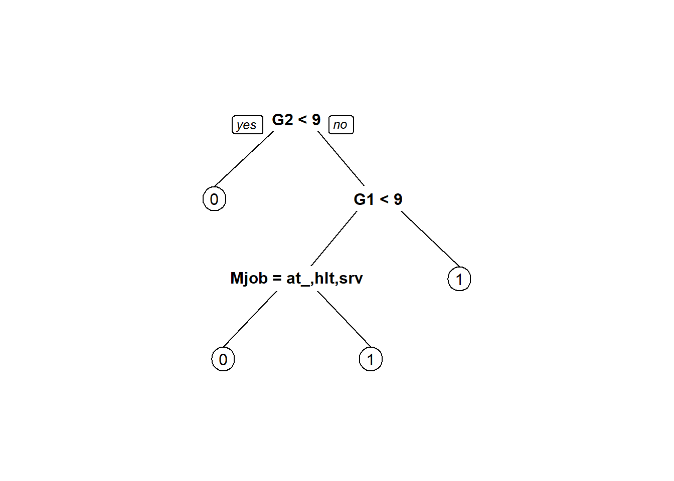
fancyRpartPlot(tree2, caption = "Classification Tree")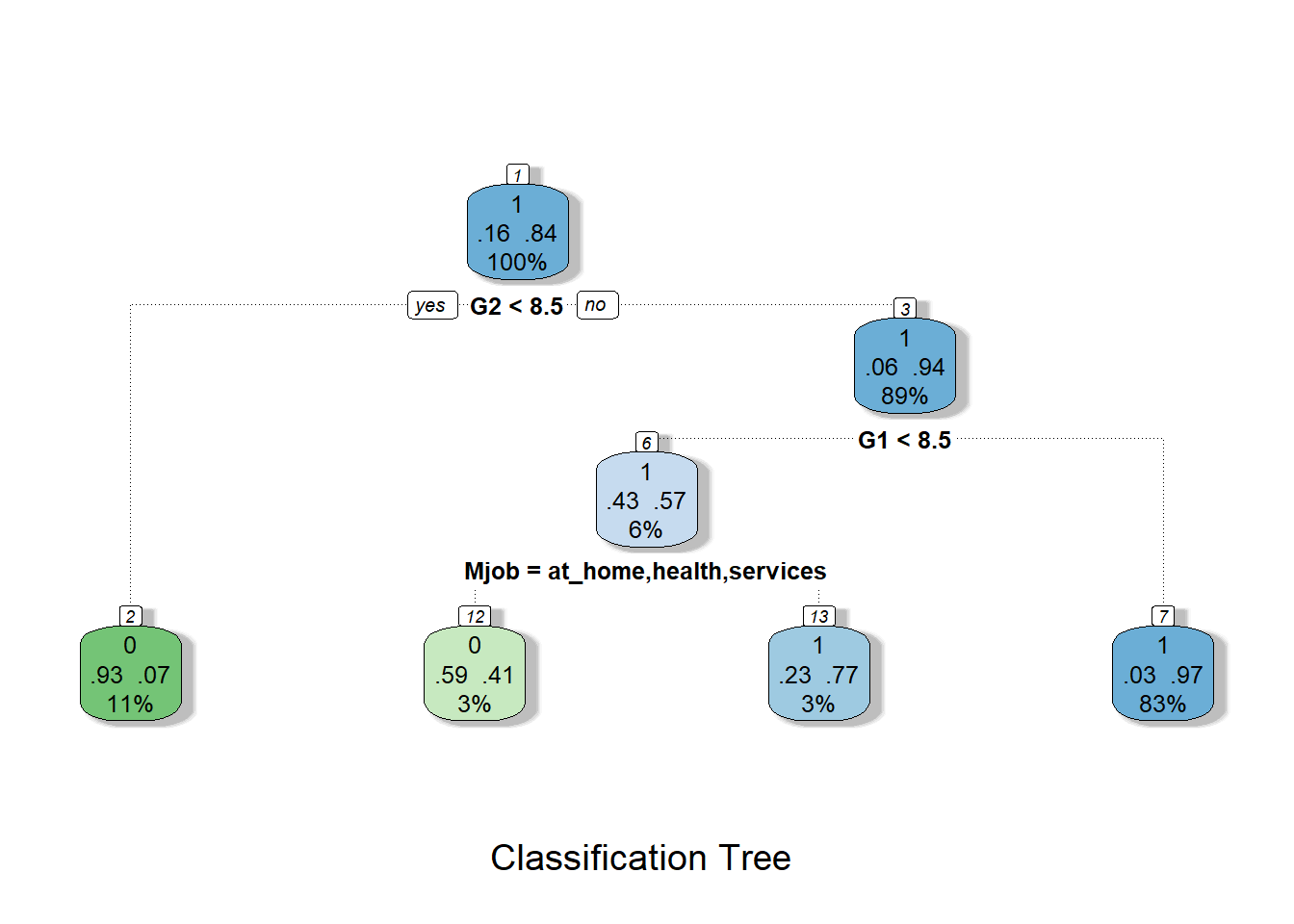
3.4.7.3 Test model
Step 25: Make predictions and confusion matrix on testing data classes, using trained model.
dtest$tree2.pred <- predict(tree2, newdata = dtest, type = 'class')
# MODIFY. change 'class' to 'prob'

(cm2 <- with(dtest,table(tree2.pred,passed)))
## passed
## tree2.pred 0 1
## 0 23 6
## 1 1 133Step 26: Make predictions and confusion matrix on testing data using probability cutoffs. Optional; results not shown.
dtest$tree2.pred <- predict(tree2, newdata = dtest, type = 'prob')

ProbabilityCutoff <- 0.5 # MODIFY. Compare different probability values.
dtest$tree2.pred.probs <- 1-dtest$tree2.pred[,1]

dtest$tree2.pred.passed <- ifelse(dtest$tree2.pred.probs > ProbabilityCutoff, 1, 0)

(cm2b <- with(dtest,table(tree2.pred.passed,passed)))
Step 27: Calculate accuracy
CorrectPredictions2 <- cm2[1,1] + cm2[2,2]
TotalStudents2 <- nrow(dtest)

(Accuracy2 <- CorrectPredictions2/TotalStudents2)
## [1] 0.9570552Step 28: Sensitivity (proportion of people who actually failed that were correctly predicted to fail)
(Sensitivity2 <- cm2[1,1]/(cm2[1,1]+cm2[2,1]))## [1] 0.9583333Step 29: Specificity (proportion of people who actually passed that were correctly predicted to pass):
(Specificity2 <- cm2[2,2]/(cm2[1,2]+cm2[2,2]))## [1] 0.9568345ALSO DOUBLE-CHECK THE CALCULATIONS ABOVE MANUALLY!
3.4.8 Logistic regression model – classification
Activity summary:
- Goal: predict binary outcome
passed, using logistic regression. - Start by using all variables to make a logistic regression model. Check predictive capability.
- Remove variables to make predictions with less information.
- Modify cutoff thresholds and see how confusion matrix changes.
- Anywhere you see the word
MODIFYis one place where you might consider making changes to the code. - Figure out which students to remediate.
3.4.8.1 Train and inspect model
Step 30: Train a logistic regression model
blr1 <- glm(passed ~ school+sex+age+address+famsize+Pstatus+Medu+Fedu+guardian+traveltime+studytime+failures+schoolsup+famsup+paid+activities+nursery+higher+internet+romantic+famrel+freetime+goout+Dalc+Walc+health+absences+Mjob+reason+Fjob+G1+G2, data=dtrain, family = "binomial")
# MODIFY. Try without G1 and G2. Then try other combinations.
# also remove variables causing multicollinearity and see if it makes a difference!

summary(blr1)
##
## Call:
## glm(formula = passed ~ school + sex + age + address + famsize +
## Pstatus + Medu + Fedu + guardian + traveltime + studytime +
## failures + schoolsup + famsup + paid + activities + nursery +
## higher + internet + romantic + famrel + freetime + goout +
## Dalc + Walc + health + absences + Mjob + reason + Fjob +
## G1 + G2, family = "binomial", data = dtrain)
##
## Deviance Residuals:
## Min 1Q Median 3Q
## -4.4822 0.0001 0.0070 0.0778
## Max
## 1.9039
##
## Coefficients:
## Estimate Std. Error
## (Intercept) -28.18719 7.74772
## schoolMS -1.97720 0.79570
## sexM -0.47597 0.79852
## age 0.68304 0.28872
## addressU -0.31461 0.76711
## famsizeLE3 -0.33865 0.67465
## PstatusT -0.34594 0.95320
## Medu 0.24135 0.34172
## Fedu -0.49910 0.33133
## guardianmother -0.50435 0.79751
## guardianother -0.51910 1.39509
## traveltime 0.43635 0.40306
## studytime -0.21295 0.41742
## failures 0.16290 0.32990
## schoolsupyes -0.13779 0.98965
## famsupyes -0.22695 0.64257
## paidyes -1.32325 1.09196
## activitiesyes 0.26279 0.60829
## nurseryyes -0.66035 0.69639
## higheryes 1.33938 0.70820
## internetyes -0.09493 0.73258
## romanticyes -1.38232 0.71817
## famrel -0.29088 0.30744
## freetime 0.09789 0.29961
## goout -0.31202 0.31968
## Dalc -0.43432 0.39008
## Walc 0.02389 0.37571
## health -0.09467 0.24009
## absences -0.03737 0.06316
## Mjobhealth -1.24837 1.30345
## Mjobother 0.06082 0.78102
## Mjobservices -0.48761 1.03117
## Mjobteacher 2.70872 1.88584
## reasonhome -0.34278 0.82103
## reasonother 0.49385 0.83244
## reasonreputation 0.48965 1.06315
## Fjobhealth -2.20526 2.10950
## Fjobother -2.03607 1.46598
## Fjobservices -0.71302 1.50363
## Fjobteacher -1.99662 2.47868
## G1 0.63381 0.22709
## G2 2.04710 0.42763
## z value Pr(>|z|)
## (Intercept) -3.638 0.000275 ***
## schoolMS -2.485 0.012960 *
## sexM -0.596 0.551135
## age 2.366 0.017995 *
## addressU -0.410 0.681717
## famsizeLE3 -0.502 0.615691
## PstatusT -0.363 0.716661
## Medu 0.706 0.480021
## Fedu -1.506 0.131970
## guardianmother -0.632 0.527118
## guardianother -0.372 0.709827
## traveltime 1.083 0.278980
## studytime -0.510 0.609938
## failures 0.494 0.621458
## schoolsupyes -0.139 0.889267
## famsupyes -0.353 0.723944
## paidyes -1.212 0.225582
## activitiesyes 0.432 0.665732
## nurseryyes -0.948 0.343003
## higheryes 1.891 0.058592 .
## internetyes -0.130 0.896901
## romanticyes -1.925 0.054257 .
## famrel -0.946 0.344092
## freetime 0.327 0.743884
## goout -0.976 0.329050
## Dalc -1.113 0.265542
## Walc 0.064 0.949305
## health -0.394 0.693361
## absences -0.592 0.554044
## Mjobhealth -0.958 0.338192
## Mjobother 0.078 0.937928
## Mjobservices -0.473 0.636309
## Mjobteacher 1.436 0.150904
## reasonhome -0.417 0.676315
## reasonother 0.593 0.553012
## reasonreputation 0.461 0.645114
## Fjobhealth -1.045 0.295839
## Fjobother -1.389 0.164870
## Fjobservices -0.474 0.635360
## Fjobteacher -0.806 0.420521
## G1 2.791 0.005254 **
## G2 4.787 1.69e-06 ***
## ---
## Signif. codes:
## 0 '***' 0.001 '**' 0.01 '*' 0.05 '.'
## 0.1 ' ' 1
##
## (Dispersion parameter for binomial family taken to be 1)
##
## Null deviance: 421.47 on 485 degrees of freedom
## Residual deviance: 118.15 on 444 degrees of freedom
## AIC: 202.15
##
## Number of Fisher Scoring iterations: 9car::vif(blr1)## GVIF Df GVIF^(1/(2*Df))
## school 2.893788 1 1.701114
## sex 2.914563 1 1.707209
## age 2.808985 1 1.676003
## address 2.564285 1 1.601338
## famsize 1.725763 1 1.313683
## Pstatus 1.844121 1 1.357984
## Medu 2.313526 1 1.521028
## Fedu 2.226737 1 1.492226
## guardian 2.707331 2 1.282730
## traveltime 2.076072 1 1.440858
## studytime 1.721130 1 1.311918
## failures 1.758342 1 1.326025
## schoolsup 1.958745 1 1.399552
## famsup 1.840819 1 1.356768
## paid 1.399295 1 1.182918
## activities 1.569459 1 1.252780
## nursery 1.497383 1 1.223676
## higher 1.709983 1 1.307663
## internet 2.098694 1 1.448687
## romantic 2.326441 1 1.525268
## famrel 1.958475 1 1.399455
## freetime 1.736687 1 1.317834
## goout 3.055775 1 1.748078
## Dalc 3.574352 1 1.890596
## Walc 4.946190 1 2.224003
## health 1.890341 1 1.374897
## absences 1.635689 1 1.278941
## Mjob 10.966200 4 1.348985
## reason 5.058090 3 1.310180
## Fjob 13.948095 4 1.390159
## G1 2.183833 1 1.477780
## G2 2.541175 1 1.5941063.4.8.2 Test model
Step 31: Make predictions on testing data, using trained model.
Predicting probabilities…
dtest$blr1.pred <- predict(blr1, newdata = dtest, type = 'response')
# MODIFY. change 'class' to 'prob'

ProbabilityCutoff <- 0.5 # MODIFY. Compare different probability values.
dtest$blr1.pred.probs <- 1-dtest$blr1.pred

dtest$blr1.pred.passed <- ifelse(dtest$blr1.pred > ProbabilityCutoff, 1, 0)

(cm3 <- with(dtest,table(blr1.pred.passed,passed)))
## passed
## blr1.pred.passed 0 1
## 0 21 4
## 1 3 135Step 32: Make confusion matrix
(cm3 <- with(dtest,table(blr1.pred.passed,passed)))## passed
## blr1.pred.passed 0 1
## 0 21 4
## 1 3 135Step 33: Calculate accuracy
CorrectPredictions3 <- cm3[1,1] + cm3[2,2]
TotalStudents3 <- nrow(dtest)

(Accuracy3 <- CorrectPredictions3/TotalStudents3)
## [1] 0.9570552Step 34: Sensitivity (proportion of people who actually failed that were correctly predicted to fail)
(Sensitivity3 <- cm3[1,1]/(cm3[1,1]+cm3[2,1]))## [1] 0.875Step 35: Specificity (proportion of people who actually passed that were correctly predicted to pass)
(Specificity3 <- cm3[2,2]/(cm3[1,2]+cm3[2,2]))## [1] 0.971223ALSO DOUBLE-CHECK THE CALCULATIONS ABOVE MANUALLY!
Step 36: It is very important for you, the data analyst, to modify the 0.5 cutoff assigned as ProbabilityCutoff above to see how you can change the predictions made by the model. Write down what you observe as you change this value and re-run the confusion matrix, accuracy, sensitivity, and specificity code above. What are the implications of your manual modification of this cutoff? Remind your instructors to discuss this, in case they forget!
3.5 Session 3: The Social Dilemma and Ethical Concerns of ML
3.5.1 Goals
Examine similarities and differences between social media analytics and HPEd analytics
Discuss ethics of predictive analytics
Practice predictive analytics research design (if time permits)
3.5.2 Discussion topics
Week 1 discussion questions related to ethics and PA/ML.
Will people start to behave differently just because they know that these models are being used to analyze them, subconsciously or consciously?
The same uses of predictive analytics shown in the movie, to make profit for the tech companies and for the people who advertise with detective companies, are also coming to Health Professions education at a very high speed. Are we ready for this?
Can we use the same technology to manipulate users for good purposes? Not only predict their outcomes but also cause them to do things to make their outcomes better? How appropriate or inappropriate is it for us to do this?
An interviewee in The Social Dilemma gave the example of Wikipedia showing different users different content based on what they were paid to show. As educators, we might show different materials to different students based on having analyzed their data. Is this the right or wrong thing to do? Who should control this capability? Should it even be possible or not?
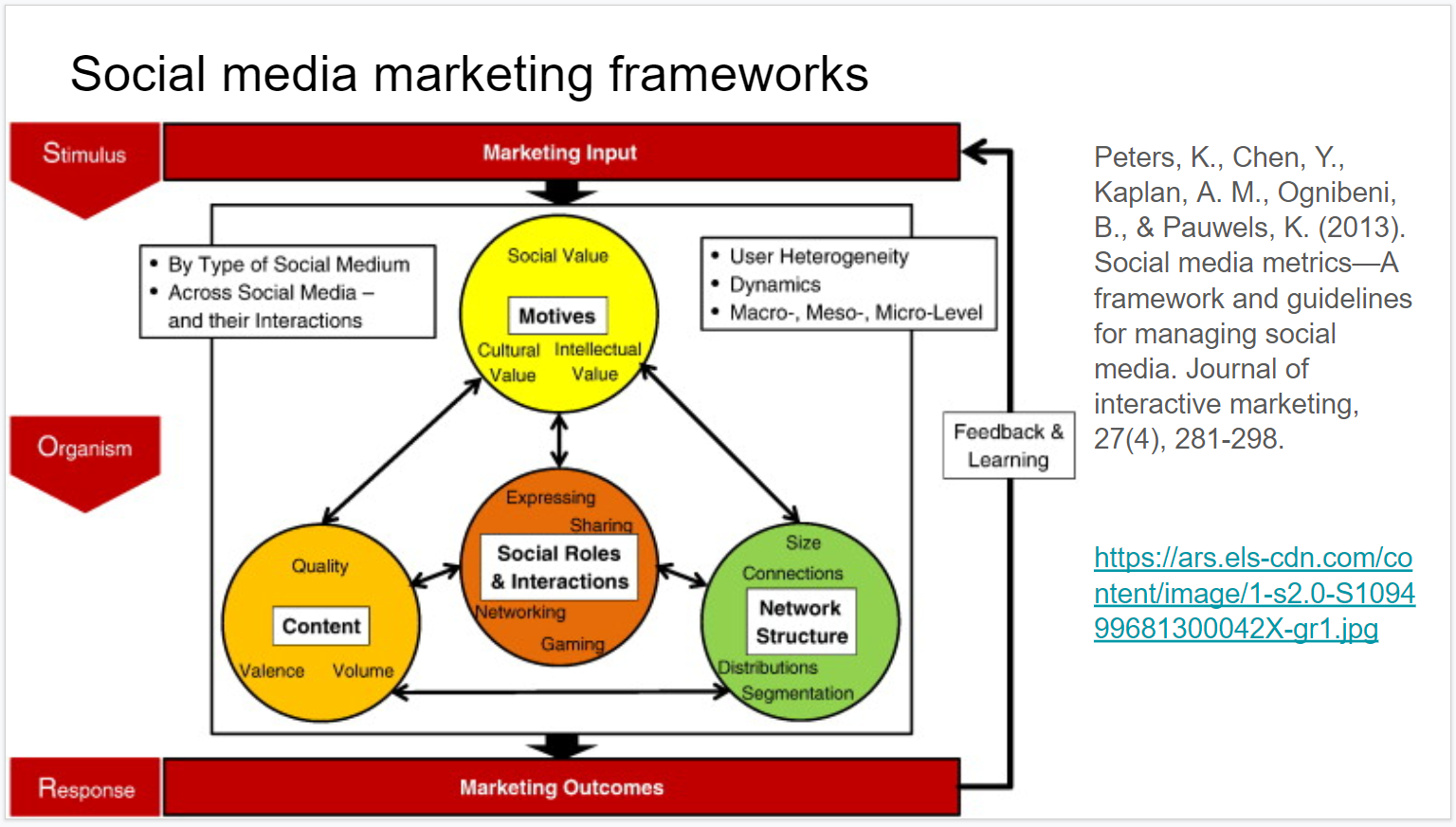
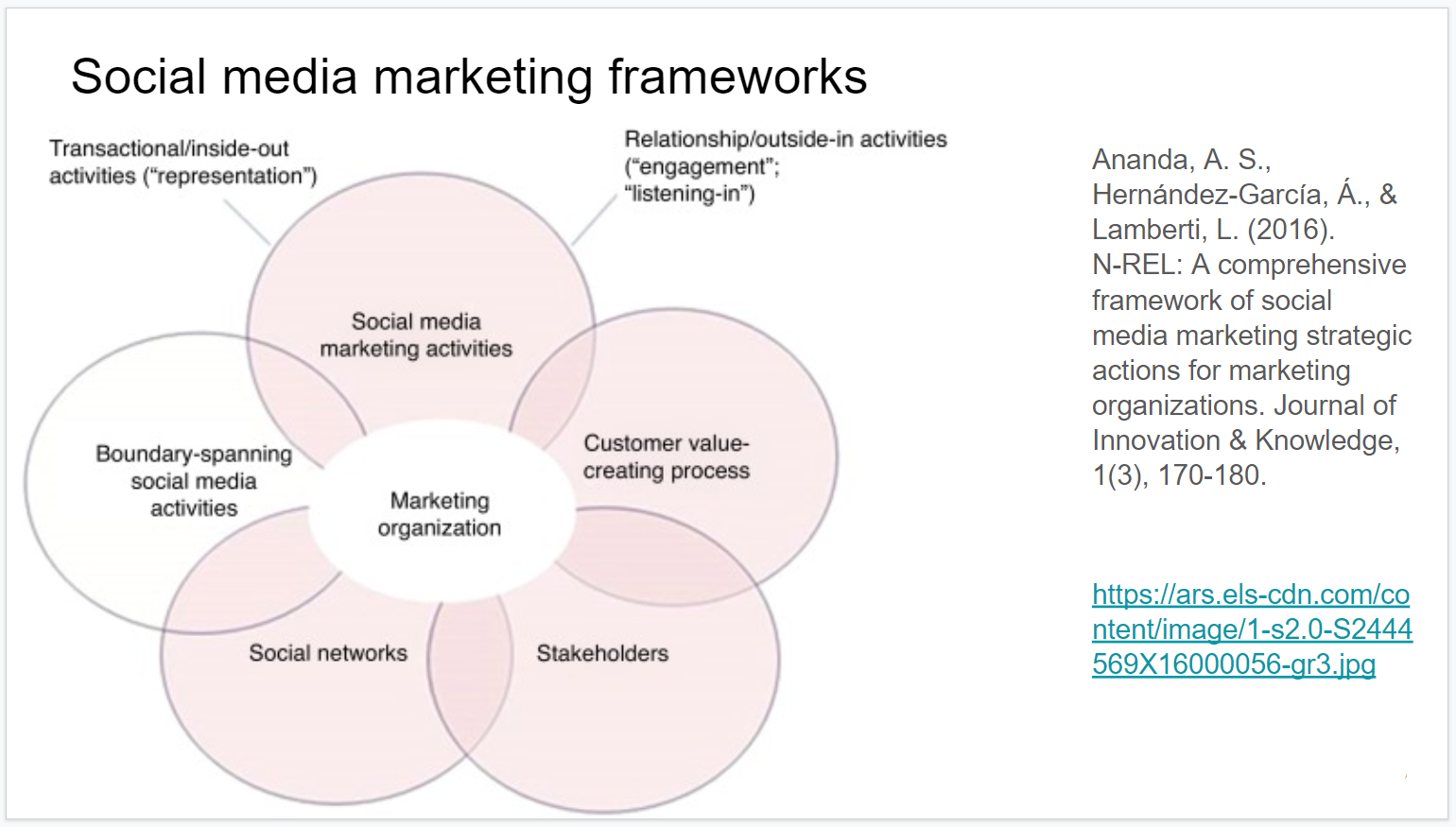
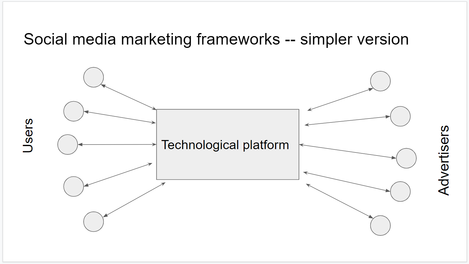
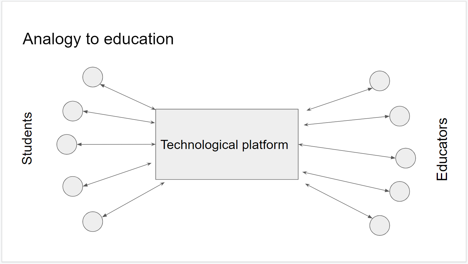
How do the social media marketing frameworks on the previous slides relate to the relationships between people and technology in HPEd?