Chapter 12 Jul 31–Aug 6: Model Validation and Evaluation in R
12.1 Goals and introduction
This week, our goals are to…
Conduct and interpret the results of k-fold cross-validation to more rigorously test the predictions of a machine learning model.
Create and interpret receiver operating characteristic (ROC) curves and associated metrics to evaluate and compare predictive models.
Calculate precision, recall, and F1 metrics to evaluate and compare predictive models.
In this chapter, we will use predictive models that we have already created earlier in the course. We will take these models and compare them against one another using the techniques outlined in the learning goals above. As always, you will then be asked to complete an assignment in which you use new (different) data to replicate the techniques that you see in the chapter. Note that this chapter only contains a few selected methods for evaluating and comparing predictive models.
12.2 Data and preparation
This chapter will once again use the mtcars dataset, as we have used in other related chapters. In this chapter, I will not demonstrate the pre-processing steps again, but you can always refer back to previous chapters—as well as your own assignments—to review how you can prepare your data. The data preparation and pre-processing that we have used before can again be used when applying the techniques demonstrated in this chapter.
Below are the few steps needed to use the mtcars data for this chapter, all of which you have seen in previous chapters:
df <- mtcars # import/copy data
df <- as.data.frame(scale(df)) # rescale all variables
df$mpg <- NULL # remove scaled mpg (dependent) variable
df$mpg <- mtcars$mpg # add raw (unscaled) mpg variable from mtcars
Now we have a single dataset with the independent variables all scaled and the dependent variable un-scaled. As you know from before, this makes the dependent variable easier to interpret when we make our predictions.
12.3 k-fold cross-validation
12.3.1 Summary of cross-validation
This section is optional to read if you feel that you already understand how cross-validation works.
So far in our course, we have always created random testing and training datasets, as subsets of our entire dataset. We then used the training data to create a predictive model and then plugged the testing data into that model to see how well it makes predictions. In this chapter, we are going to use the same logic of training and testing that we did before, but we are going to make multiple testing and training datasets out of our entire dataset, such that all observations are in the testing dataset once.
To do this, we will use a method called k-fold cross-validation.47 k represents the number of “folds”—or groups—into which we will divide our data. We will choose a value of k that best fits our needs in each analytics situation. However, a commonly selected value for k is 10. In this chapter, we will conduct 10-fold cross-validation. This means that we will divide our data up into 10 separate groups. The dataset we are using in this chapter has 32 observations (cars). 32 divided by 10 is 3.2, which is in between 3 and 4, this means that we will make 10 groups (also called folds), each of which has 3 or 4 observations in it.
Once we have 10 groups, we can number each of these groups from 1 to 10. Remember that in this case, each group contains 3 or 4 observations (cars), approximately 10% of the total data. Keep in mind that we should randomly assign observations to each group (we should not just put the first 3 observations in the data into group #1, the next 4 observations into group #2, and so on).
Here is how we will use these 10 folds/groups of our data:
- Use group #1 as the testing data and use combined groups #2-10 as the training data. Create a predictive model using the training data and then see how well it makes predictions on the testing data, just like we always have done. Save the results of the predictions made on group #1.
- Use group #2 as the testing data and use combined groups #1 and #3-10 as the training data. Create a predictive model using the training data and then see how well it makes predictions on the testing data, just like we always have done. Save the results of the predictions made on group #2.
- Use group #3 as the testing data and use combined groups #1-2 and #4-10 as the training data. Create a predictive model using the training data and then see how well it makes predictions on the testing data, just like we always have done. Save the results of the predictions made on group #3.
- Continue this procedure until each of the 10 groups has been used one time as the testing data. Each time we use another group as the testing data, we will save the predictions made by the model.
- Compare the saved actual and predicted values for all observations, keeping in mind that the predictions for a given observation were made when it was part of the testing data.
In the procedure above, we used a single predictive method, but we created 10 different models with it. We will now go through the procedure described above, before further unpacking it in detail. If the information above did not fully make sense yet, that is fine. I think that seeing the procedure conducted below will help clarify what is happening.
12.3.2 Assign groups/folds
We will now begin the process described above. The first step is to randomly create our 10 groups.
Before we make the groups, let’s quickly look at our data in its initial form:
df## cyl
## Mazda RX4 -0.1049878
## Mazda RX4 Wag -0.1049878
## Datsun 710 -1.2248578
## Hornet 4 Drive -0.1049878
## Hornet Sportabout 1.0148821
## Valiant -0.1049878
## Duster 360 1.0148821
## Merc 240D -1.2248578
## Merc 230 -1.2248578
## Merc 280 -0.1049878
## Merc 280C -0.1049878
## Merc 450SE 1.0148821
## Merc 450SL 1.0148821
## Merc 450SLC 1.0148821
## Cadillac Fleetwood 1.0148821
## Lincoln Continental 1.0148821
## Chrysler Imperial 1.0148821
## Fiat 128 -1.2248578
## Honda Civic -1.2248578
## Toyota Corolla -1.2248578
## Toyota Corona -1.2248578
## Dodge Challenger 1.0148821
## AMC Javelin 1.0148821
## Camaro Z28 1.0148821
## Pontiac Firebird 1.0148821
## Fiat X1-9 -1.2248578
## Porsche 914-2 -1.2248578
## Lotus Europa -1.2248578
## Ford Pantera L 1.0148821
## Ferrari Dino -0.1049878
## Maserati Bora 1.0148821
## Volvo 142E -1.2248578
## disp
## Mazda RX4 -0.57061982
## Mazda RX4 Wag -0.57061982
## Datsun 710 -0.99018209
## Hornet 4 Drive 0.22009369
## Hornet Sportabout 1.04308123
## Valiant -0.04616698
## Duster 360 1.04308123
## Merc 240D -0.67793094
## Merc 230 -0.72553512
## Merc 280 -0.50929918
## Merc 280C -0.50929918
## Merc 450SE 0.36371309
## Merc 450SL 0.36371309
## Merc 450SLC 0.36371309
## Cadillac Fleetwood 1.94675381
## Lincoln Continental 1.84993175
## Chrysler Imperial 1.68856165
## Fiat 128 -1.22658929
## Honda Civic -1.25079481
## Toyota Corolla -1.28790993
## Toyota Corona -0.89255318
## Dodge Challenger 0.70420401
## AMC Javelin 0.59124494
## Camaro Z28 0.96239618
## Pontiac Firebird 1.36582144
## Fiat X1-9 -1.22416874
## Porsche 914-2 -0.89093948
## Lotus Europa -1.09426581
## Ford Pantera L 0.97046468
## Ferrari Dino -0.69164740
## Maserati Bora 0.56703942
## Volvo 142E -0.88529152
## hp
## Mazda RX4 -0.53509284
## Mazda RX4 Wag -0.53509284
## Datsun 710 -0.78304046
## Hornet 4 Drive -0.53509284
## Hornet Sportabout 0.41294217
## Valiant -0.60801861
## Duster 360 1.43390296
## Merc 240D -1.23518023
## Merc 230 -0.75387015
## Merc 280 -0.34548584
## Merc 280C -0.34548584
## Merc 450SE 0.48586794
## Merc 450SL 0.48586794
## Merc 450SLC 0.48586794
## Cadillac Fleetwood 0.85049680
## Lincoln Continental 0.99634834
## Chrysler Imperial 1.21512565
## Fiat 128 -1.17683962
## Honda Civic -1.38103178
## Toyota Corolla -1.19142477
## Toyota Corona -0.72469984
## Dodge Challenger 0.04831332
## AMC Javelin 0.04831332
## Camaro Z28 1.43390296
## Pontiac Firebird 0.41294217
## Fiat X1-9 -1.17683962
## Porsche 914-2 -0.81221077
## Lotus Europa -0.49133738
## Ford Pantera L 1.71102089
## Ferrari Dino 0.41294217
## Maserati Bora 2.74656682
## Volvo 142E -0.54967799
## drat
## Mazda RX4 0.56751369
## Mazda RX4 Wag 0.56751369
## Datsun 710 0.47399959
## Hornet 4 Drive -0.96611753
## Hornet Sportabout -0.83519779
## Valiant -1.56460776
## Duster 360 -0.72298087
## Merc 240D 0.17475447
## Merc 230 0.60491932
## Merc 280 0.60491932
## Merc 280C 0.60491932
## Merc 450SE -0.98482035
## Merc 450SL -0.98482035
## Merc 450SLC -0.98482035
## Cadillac Fleetwood -1.24665983
## Lincoln Continental -1.11574009
## Chrysler Imperial -0.68557523
## Fiat 128 0.90416444
## Honda Civic 2.49390411
## Toyota Corolla 1.16600392
## Toyota Corona 0.19345729
## Dodge Challenger -1.56460776
## AMC Javelin -0.83519779
## Camaro Z28 0.24956575
## Pontiac Firebird -0.96611753
## Fiat X1-9 0.90416444
## Porsche 914-2 1.55876313
## Lotus Europa 0.32437703
## Ford Pantera L 1.16600392
## Ferrari Dino 0.04383473
## Maserati Bora -0.10578782
## Volvo 142E 0.96027290
## wt
## Mazda RX4 -0.610399567
## Mazda RX4 Wag -0.349785269
## Datsun 710 -0.917004624
## Hornet 4 Drive -0.002299538
## Hornet Sportabout 0.227654255
## Valiant 0.248094592
## Duster 360 0.360516446
## Merc 240D -0.027849959
## Merc 230 -0.068730634
## Merc 280 0.227654255
## Merc 280C 0.227654255
## Merc 450SE 0.871524874
## Merc 450SL 0.524039143
## Merc 450SLC 0.575139986
## Cadillac Fleetwood 2.077504765
## Lincoln Continental 2.255335698
## Chrysler Imperial 2.174596366
## Fiat 128 -1.039646647
## Honda Civic -1.637526508
## Toyota Corolla -1.412682800
## Toyota Corona -0.768812180
## Dodge Challenger 0.309415603
## AMC Javelin 0.222544170
## Camaro Z28 0.636460997
## Pontiac Firebird 0.641571082
## Fiat X1-9 -1.310481114
## Porsche 914-2 -1.100967659
## Lotus Europa -1.741772228
## Ford Pantera L -0.048290296
## Ferrari Dino -0.457097039
## Maserati Bora 0.360516446
## Volvo 142E -0.446876870
## qsec
## Mazda RX4 -0.77716515
## Mazda RX4 Wag -0.46378082
## Datsun 710 0.42600682
## Hornet 4 Drive 0.89048716
## Hornet Sportabout -0.46378082
## Valiant 1.32698675
## Duster 360 -1.12412636
## Merc 240D 1.20387148
## Merc 230 2.82675459
## Merc 280 0.25252621
## Merc 280C 0.58829513
## Merc 450SE -0.25112717
## Merc 450SL -0.13920420
## Merc 450SLC 0.08464175
## Cadillac Fleetwood 0.07344945
## Lincoln Continental -0.01608893
## Chrysler Imperial -0.23993487
## Fiat 128 0.90727560
## Honda Civic 0.37564148
## Toyota Corolla 1.14790999
## Toyota Corona 1.20946763
## Dodge Challenger -0.54772305
## AMC Javelin -0.30708866
## Camaro Z28 -1.36476075
## Pontiac Firebird -0.44699237
## Fiat X1-9 0.58829513
## Porsche 914-2 -0.64285758
## Lotus Europa -0.53093460
## Ford Pantera L -1.87401028
## Ferrari Dino -1.31439542
## Maserati Bora -1.81804880
## Volvo 142E 0.42041067
## vs am
## Mazda RX4 -0.8680278 1.1899014
## Mazda RX4 Wag -0.8680278 1.1899014
## Datsun 710 1.1160357 1.1899014
## Hornet 4 Drive 1.1160357 -0.8141431
## Hornet Sportabout -0.8680278 -0.8141431
## Valiant 1.1160357 -0.8141431
## Duster 360 -0.8680278 -0.8141431
## Merc 240D 1.1160357 -0.8141431
## Merc 230 1.1160357 -0.8141431
## Merc 280 1.1160357 -0.8141431
## Merc 280C 1.1160357 -0.8141431
## Merc 450SE -0.8680278 -0.8141431
## Merc 450SL -0.8680278 -0.8141431
## Merc 450SLC -0.8680278 -0.8141431
## Cadillac Fleetwood -0.8680278 -0.8141431
## Lincoln Continental -0.8680278 -0.8141431
## Chrysler Imperial -0.8680278 -0.8141431
## Fiat 128 1.1160357 1.1899014
## Honda Civic 1.1160357 1.1899014
## Toyota Corolla 1.1160357 1.1899014
## Toyota Corona 1.1160357 -0.8141431
## Dodge Challenger -0.8680278 -0.8141431
## AMC Javelin -0.8680278 -0.8141431
## Camaro Z28 -0.8680278 -0.8141431
## Pontiac Firebird -0.8680278 -0.8141431
## Fiat X1-9 1.1160357 1.1899014
## Porsche 914-2 -0.8680278 1.1899014
## Lotus Europa 1.1160357 1.1899014
## Ford Pantera L -0.8680278 1.1899014
## Ferrari Dino -0.8680278 1.1899014
## Maserati Bora -0.8680278 1.1899014
## Volvo 142E 1.1160357 1.1899014
## gear carb
## Mazda RX4 0.4235542 0.7352031
## Mazda RX4 Wag 0.4235542 0.7352031
## Datsun 710 0.4235542 -1.1221521
## Hornet 4 Drive -0.9318192 -1.1221521
## Hornet Sportabout -0.9318192 -0.5030337
## Valiant -0.9318192 -1.1221521
## Duster 360 -0.9318192 0.7352031
## Merc 240D 0.4235542 -0.5030337
## Merc 230 0.4235542 -0.5030337
## Merc 280 0.4235542 0.7352031
## Merc 280C 0.4235542 0.7352031
## Merc 450SE -0.9318192 0.1160847
## Merc 450SL -0.9318192 0.1160847
## Merc 450SLC -0.9318192 0.1160847
## Cadillac Fleetwood -0.9318192 0.7352031
## Lincoln Continental -0.9318192 0.7352031
## Chrysler Imperial -0.9318192 0.7352031
## Fiat 128 0.4235542 -1.1221521
## Honda Civic 0.4235542 -0.5030337
## Toyota Corolla 0.4235542 -1.1221521
## Toyota Corona -0.9318192 -1.1221521
## Dodge Challenger -0.9318192 -0.5030337
## AMC Javelin -0.9318192 -0.5030337
## Camaro Z28 -0.9318192 0.7352031
## Pontiac Firebird -0.9318192 -0.5030337
## Fiat X1-9 0.4235542 -1.1221521
## Porsche 914-2 1.7789276 -0.5030337
## Lotus Europa 1.7789276 -0.5030337
## Ford Pantera L 1.7789276 0.7352031
## Ferrari Dino 1.7789276 1.9734398
## Maserati Bora 1.7789276 3.2116766
## Volvo 142E 0.4235542 -0.5030337
## mpg
## Mazda RX4 21.0
## Mazda RX4 Wag 21.0
## Datsun 710 22.8
## Hornet 4 Drive 21.4
## Hornet Sportabout 18.7
## Valiant 18.1
## Duster 360 14.3
## Merc 240D 24.4
## Merc 230 22.8
## Merc 280 19.2
## Merc 280C 17.8
## Merc 450SE 16.4
## Merc 450SL 17.3
## Merc 450SLC 15.2
## Cadillac Fleetwood 10.4
## Lincoln Continental 10.4
## Chrysler Imperial 14.7
## Fiat 128 32.4
## Honda Civic 30.4
## Toyota Corolla 33.9
## Toyota Corona 21.5
## Dodge Challenger 15.5
## AMC Javelin 15.2
## Camaro Z28 13.3
## Pontiac Firebird 19.2
## Fiat X1-9 27.3
## Porsche 914-2 26.0
## Lotus Europa 30.4
## Ford Pantera L 15.8
## Ferrari Dino 19.7
## Maserati Bora 15.0
## Volvo 142E 21.4As you can see above, we are once again dealing with the mtcars data that we have used before. We have renamed the data as df.
As a first step towards assigning groups, let’s randomly reorder the data with the code below:
df <- df[sample(1:nrow(df)), ]The code above is simply creating a new dataset (which we are also calling df, and it will replace the previous version of df) which is created by randomly sampling from the old dataset. This random sampling is done without replacement, such that each observation in the old data is only selected into the new data one time.
Now that our data is randomly reordered, we will tell R how many groups we want to divide the data into:
k <- 10 # assign number of groups/foldsAbove, we assigned k to be equal to the number 10. For the rest of this chapter, anywhere we type k, it will represent the number 10. The reason we assign k to represent 10 instead of just typing 10 throughout our code is that we may later want to change the number of groups that we create. Making that change will be much easier if all we have to do is go to the top of our code and change k to a different number, in the line of code above.
Within R, let’s calculate how big each group should be:
groupsize <- nrow(df)/kAbove, we assigned groupsize to be equal to the result of the number of observations in our data divided by the number of groups that we want. We already know that in this situation the value of groupsize will be equal to 3.2. But again, we want this code to work with any data that we may want to use. Therefore, it is best if we can program R to calculate group size for us automatically.
Next, we will give each observation an identification number, since these are not already provided in the data:
df$idnum <- seq(1:nrow(df))Above, we created a new variable called idnum which will just be the row number of each observation. We created this identification number by assigning idnum to be equal to the value of a sequence of numbers counting upwards from 1 until the number of observations in the data.
Finally, we can assign a group number to each observation:
df$group <- ceiling(df$idnum/groupsize)Above, we created a new variable called group, which will have a value between 1 and 10 and will determine each observation’s membership in a group. The ceiling function is used to round any non-integer numbers up (never down) to the nearest integer. In the code above, we took each observation’s identification number and divided it by the ideal group size, which in this case is 3.2. In most cases, that quotient will be a non-integer number. Since we don’t want any groups to be identified by non-integer numbers, we round these non-integer quotients up to the closest whole number.
Now that we have made all the changes described above, let’s once again inspect our data in its new form:
df## cyl
## Chrysler Imperial 1.0148821
## Dodge Challenger 1.0148821
## Lincoln Continental 1.0148821
## Merc 450SL 1.0148821
## Hornet Sportabout 1.0148821
## AMC Javelin 1.0148821
## Pontiac Firebird 1.0148821
## Cadillac Fleetwood 1.0148821
## Merc 450SLC 1.0148821
## Camaro Z28 1.0148821
## Merc 240D -1.2248578
## Toyota Corona -1.2248578
## Mazda RX4 Wag -0.1049878
## Porsche 914-2 -1.2248578
## Ferrari Dino -0.1049878
## Toyota Corolla -1.2248578
## Datsun 710 -1.2248578
## Fiat X1-9 -1.2248578
## Maserati Bora 1.0148821
## Volvo 142E -1.2248578
## Merc 450SE 1.0148821
## Mazda RX4 -0.1049878
## Hornet 4 Drive -0.1049878
## Lotus Europa -1.2248578
## Honda Civic -1.2248578
## Valiant -0.1049878
## Merc 280 -0.1049878
## Merc 230 -1.2248578
## Ford Pantera L 1.0148821
## Merc 280C -0.1049878
## Fiat 128 -1.2248578
## Duster 360 1.0148821
## disp
## Chrysler Imperial 1.68856165
## Dodge Challenger 0.70420401
## Lincoln Continental 1.84993175
## Merc 450SL 0.36371309
## Hornet Sportabout 1.04308123
## AMC Javelin 0.59124494
## Pontiac Firebird 1.36582144
## Cadillac Fleetwood 1.94675381
## Merc 450SLC 0.36371309
## Camaro Z28 0.96239618
## Merc 240D -0.67793094
## Toyota Corona -0.89255318
## Mazda RX4 Wag -0.57061982
## Porsche 914-2 -0.89093948
## Ferrari Dino -0.69164740
## Toyota Corolla -1.28790993
## Datsun 710 -0.99018209
## Fiat X1-9 -1.22416874
## Maserati Bora 0.56703942
## Volvo 142E -0.88529152
## Merc 450SE 0.36371309
## Mazda RX4 -0.57061982
## Hornet 4 Drive 0.22009369
## Lotus Europa -1.09426581
## Honda Civic -1.25079481
## Valiant -0.04616698
## Merc 280 -0.50929918
## Merc 230 -0.72553512
## Ford Pantera L 0.97046468
## Merc 280C -0.50929918
## Fiat 128 -1.22658929
## Duster 360 1.04308123
## hp
## Chrysler Imperial 1.21512565
## Dodge Challenger 0.04831332
## Lincoln Continental 0.99634834
## Merc 450SL 0.48586794
## Hornet Sportabout 0.41294217
## AMC Javelin 0.04831332
## Pontiac Firebird 0.41294217
## Cadillac Fleetwood 0.85049680
## Merc 450SLC 0.48586794
## Camaro Z28 1.43390296
## Merc 240D -1.23518023
## Toyota Corona -0.72469984
## Mazda RX4 Wag -0.53509284
## Porsche 914-2 -0.81221077
## Ferrari Dino 0.41294217
## Toyota Corolla -1.19142477
## Datsun 710 -0.78304046
## Fiat X1-9 -1.17683962
## Maserati Bora 2.74656682
## Volvo 142E -0.54967799
## Merc 450SE 0.48586794
## Mazda RX4 -0.53509284
## Hornet 4 Drive -0.53509284
## Lotus Europa -0.49133738
## Honda Civic -1.38103178
## Valiant -0.60801861
## Merc 280 -0.34548584
## Merc 230 -0.75387015
## Ford Pantera L 1.71102089
## Merc 280C -0.34548584
## Fiat 128 -1.17683962
## Duster 360 1.43390296
## drat
## Chrysler Imperial -0.68557523
## Dodge Challenger -1.56460776
## Lincoln Continental -1.11574009
## Merc 450SL -0.98482035
## Hornet Sportabout -0.83519779
## AMC Javelin -0.83519779
## Pontiac Firebird -0.96611753
## Cadillac Fleetwood -1.24665983
## Merc 450SLC -0.98482035
## Camaro Z28 0.24956575
## Merc 240D 0.17475447
## Toyota Corona 0.19345729
## Mazda RX4 Wag 0.56751369
## Porsche 914-2 1.55876313
## Ferrari Dino 0.04383473
## Toyota Corolla 1.16600392
## Datsun 710 0.47399959
## Fiat X1-9 0.90416444
## Maserati Bora -0.10578782
## Volvo 142E 0.96027290
## Merc 450SE -0.98482035
## Mazda RX4 0.56751369
## Hornet 4 Drive -0.96611753
## Lotus Europa 0.32437703
## Honda Civic 2.49390411
## Valiant -1.56460776
## Merc 280 0.60491932
## Merc 230 0.60491932
## Ford Pantera L 1.16600392
## Merc 280C 0.60491932
## Fiat 128 0.90416444
## Duster 360 -0.72298087
## wt
## Chrysler Imperial 2.174596366
## Dodge Challenger 0.309415603
## Lincoln Continental 2.255335698
## Merc 450SL 0.524039143
## Hornet Sportabout 0.227654255
## AMC Javelin 0.222544170
## Pontiac Firebird 0.641571082
## Cadillac Fleetwood 2.077504765
## Merc 450SLC 0.575139986
## Camaro Z28 0.636460997
## Merc 240D -0.027849959
## Toyota Corona -0.768812180
## Mazda RX4 Wag -0.349785269
## Porsche 914-2 -1.100967659
## Ferrari Dino -0.457097039
## Toyota Corolla -1.412682800
## Datsun 710 -0.917004624
## Fiat X1-9 -1.310481114
## Maserati Bora 0.360516446
## Volvo 142E -0.446876870
## Merc 450SE 0.871524874
## Mazda RX4 -0.610399567
## Hornet 4 Drive -0.002299538
## Lotus Europa -1.741772228
## Honda Civic -1.637526508
## Valiant 0.248094592
## Merc 280 0.227654255
## Merc 230 -0.068730634
## Ford Pantera L -0.048290296
## Merc 280C 0.227654255
## Fiat 128 -1.039646647
## Duster 360 0.360516446
## qsec
## Chrysler Imperial -0.23993487
## Dodge Challenger -0.54772305
## Lincoln Continental -0.01608893
## Merc 450SL -0.13920420
## Hornet Sportabout -0.46378082
## AMC Javelin -0.30708866
## Pontiac Firebird -0.44699237
## Cadillac Fleetwood 0.07344945
## Merc 450SLC 0.08464175
## Camaro Z28 -1.36476075
## Merc 240D 1.20387148
## Toyota Corona 1.20946763
## Mazda RX4 Wag -0.46378082
## Porsche 914-2 -0.64285758
## Ferrari Dino -1.31439542
## Toyota Corolla 1.14790999
## Datsun 710 0.42600682
## Fiat X1-9 0.58829513
## Maserati Bora -1.81804880
## Volvo 142E 0.42041067
## Merc 450SE -0.25112717
## Mazda RX4 -0.77716515
## Hornet 4 Drive 0.89048716
## Lotus Europa -0.53093460
## Honda Civic 0.37564148
## Valiant 1.32698675
## Merc 280 0.25252621
## Merc 230 2.82675459
## Ford Pantera L -1.87401028
## Merc 280C 0.58829513
## Fiat 128 0.90727560
## Duster 360 -1.12412636
## vs am
## Chrysler Imperial -0.8680278 -0.8141431
## Dodge Challenger -0.8680278 -0.8141431
## Lincoln Continental -0.8680278 -0.8141431
## Merc 450SL -0.8680278 -0.8141431
## Hornet Sportabout -0.8680278 -0.8141431
## AMC Javelin -0.8680278 -0.8141431
## Pontiac Firebird -0.8680278 -0.8141431
## Cadillac Fleetwood -0.8680278 -0.8141431
## Merc 450SLC -0.8680278 -0.8141431
## Camaro Z28 -0.8680278 -0.8141431
## Merc 240D 1.1160357 -0.8141431
## Toyota Corona 1.1160357 -0.8141431
## Mazda RX4 Wag -0.8680278 1.1899014
## Porsche 914-2 -0.8680278 1.1899014
## Ferrari Dino -0.8680278 1.1899014
## Toyota Corolla 1.1160357 1.1899014
## Datsun 710 1.1160357 1.1899014
## Fiat X1-9 1.1160357 1.1899014
## Maserati Bora -0.8680278 1.1899014
## Volvo 142E 1.1160357 1.1899014
## Merc 450SE -0.8680278 -0.8141431
## Mazda RX4 -0.8680278 1.1899014
## Hornet 4 Drive 1.1160357 -0.8141431
## Lotus Europa 1.1160357 1.1899014
## Honda Civic 1.1160357 1.1899014
## Valiant 1.1160357 -0.8141431
## Merc 280 1.1160357 -0.8141431
## Merc 230 1.1160357 -0.8141431
## Ford Pantera L -0.8680278 1.1899014
## Merc 280C 1.1160357 -0.8141431
## Fiat 128 1.1160357 1.1899014
## Duster 360 -0.8680278 -0.8141431
## gear carb
## Chrysler Imperial -0.9318192 0.7352031
## Dodge Challenger -0.9318192 -0.5030337
## Lincoln Continental -0.9318192 0.7352031
## Merc 450SL -0.9318192 0.1160847
## Hornet Sportabout -0.9318192 -0.5030337
## AMC Javelin -0.9318192 -0.5030337
## Pontiac Firebird -0.9318192 -0.5030337
## Cadillac Fleetwood -0.9318192 0.7352031
## Merc 450SLC -0.9318192 0.1160847
## Camaro Z28 -0.9318192 0.7352031
## Merc 240D 0.4235542 -0.5030337
## Toyota Corona -0.9318192 -1.1221521
## Mazda RX4 Wag 0.4235542 0.7352031
## Porsche 914-2 1.7789276 -0.5030337
## Ferrari Dino 1.7789276 1.9734398
## Toyota Corolla 0.4235542 -1.1221521
## Datsun 710 0.4235542 -1.1221521
## Fiat X1-9 0.4235542 -1.1221521
## Maserati Bora 1.7789276 3.2116766
## Volvo 142E 0.4235542 -0.5030337
## Merc 450SE -0.9318192 0.1160847
## Mazda RX4 0.4235542 0.7352031
## Hornet 4 Drive -0.9318192 -1.1221521
## Lotus Europa 1.7789276 -0.5030337
## Honda Civic 0.4235542 -0.5030337
## Valiant -0.9318192 -1.1221521
## Merc 280 0.4235542 0.7352031
## Merc 230 0.4235542 -0.5030337
## Ford Pantera L 1.7789276 0.7352031
## Merc 280C 0.4235542 0.7352031
## Fiat 128 0.4235542 -1.1221521
## Duster 360 -0.9318192 0.7352031
## mpg idnum group
## Chrysler Imperial 14.7 1 1
## Dodge Challenger 15.5 2 1
## Lincoln Continental 10.4 3 1
## Merc 450SL 17.3 4 2
## Hornet Sportabout 18.7 5 2
## AMC Javelin 15.2 6 2
## Pontiac Firebird 19.2 7 3
## Cadillac Fleetwood 10.4 8 3
## Merc 450SLC 15.2 9 3
## Camaro Z28 13.3 10 4
## Merc 240D 24.4 11 4
## Toyota Corona 21.5 12 4
## Mazda RX4 Wag 21.0 13 5
## Porsche 914-2 26.0 14 5
## Ferrari Dino 19.7 15 5
## Toyota Corolla 33.9 16 5
## Datsun 710 22.8 17 6
## Fiat X1-9 27.3 18 6
## Maserati Bora 15.0 19 6
## Volvo 142E 21.4 20 7
## Merc 450SE 16.4 21 7
## Mazda RX4 21.0 22 7
## Hornet 4 Drive 21.4 23 8
## Lotus Europa 30.4 24 8
## Honda Civic 30.4 25 8
## Valiant 18.1 26 9
## Merc 280 19.2 27 9
## Merc 230 22.8 28 9
## Ford Pantera L 15.8 29 10
## Merc 280C 17.8 30 10
## Fiat 128 32.4 31 10
## Duster 360 14.3 32 10By inspecting the data above, you can see all of the changes that we made just now:
- The observations have been randomly reordered.
- There is a new variable called
idnumwhich gives each Observation a unique identification number. - There is a new variable called
groupwhich identifies which of the 10 groups each observation is a member of. Each group contains three or four observations. These observations were randomly assigned because we randomly re-sorted the data before we assigned the groups.
We have completed the process of randomly dividing our data into 10 groups. We are now ready to create a cross-validated predictive model.
12.3.3 Run cross-validated model
We will now follow the procedure described earlier to create a cross-validated predictive model. It is important to note that the code below is not the only way to accomplish this technique.
We will start by creating an empty dataset called dfinal:
dfinal <- df[-c(1:nrow(df)),] # make empty datasetThe code above takes the existing dataset df and removes all of its rows (observations), but it keeps the column headers (the variable names). You can think of dfinal as a “container” into which we are going to put all of the predictions as we make them throughout the cross-validation process. You will see this process in action shortly.
Let’s inspect the empty dataset that we just made:
dim(dfinal)## [1] 0 13From the output above, you can see that dfinal has 0 observations (rows) but it does have some variables (columns).
And we can see what those variables are:
names(dfinal)## [1] "cyl" "disp" "hp" "drat"
## [5] "wt" "qsec" "vs" "am"
## [9] "gear" "carb" "mpg" "idnum"
## [13] "group"The first type of model that we will run using this cross-validation technique is a random forest model. To run this model, we need to load the appropriate package:
if(!require(randomForest)) install.packages('randomForest')
library(randomForest)
We are now ready to conduct the cross-validation procedure and save the predicted results. As you already know, to do this, we will have to run a random forest model 10 different times. Each time, the training and testing data will be different. To repeat the procedure 10 times, we will use what is called a loop. More specifically, the type of loop we are using is called a for loop. A for loop is a tool that we can add to our code that will repeat a procedure as many times as we specify, over and over again.
Here is the loop to run our random forest model 10 times:
for(i in 1:k) {
  cat("\n=== Repetition",i,"===\n\n")
  dtest <- df[df$group==i,]
  dtrain <- df[df$group!=i,]
  dtrain$group <- NULL
  dtrain$idnum <- NULL
  rf1 <- randomForest(mpg ~ .,data=dtrain, proximity=TRUE,ntree=1000)
  dtest$rf.pred <- predict(rf1, newdata = dtest)
  print(dtest[c("idnum","group","mpg","rf.pred")])
  dfinal <- rbind(dfinal,dtest)
}
##
## === Repetition 1 ===
##
## idnum group mpg
## Chrysler Imperial 1 1 14.7
## Dodge Challenger 2 1 15.5
## Lincoln Continental 3 1 10.4
## rf.pred
## Chrysler Imperial 13.77015
## Dodge Challenger 16.74743
## Lincoln Continental 12.95552
##
## === Repetition 2 ===
##
## idnum group mpg
## Merc 450SL 4 2 17.3
## Hornet Sportabout 5 2 18.7
## AMC Javelin 6 2 15.2
## rf.pred
## Merc 450SL 15.79006
## Hornet Sportabout 17.27735
## AMC Javelin 17.25699
##
## === Repetition 3 ===
##
## idnum group mpg
## Pontiac Firebird 7 3 19.2
## Cadillac Fleetwood 8 3 10.4
## Merc 450SLC 9 3 15.2
## rf.pred
## Pontiac Firebird 16.37992
## Cadillac Fleetwood 13.11582
## Merc 450SLC 16.10666
##
## === Repetition 4 ===
##
## idnum group mpg rf.pred
## Camaro Z28 10 4 13.3 15.49644
## Merc 240D 11 4 24.4 23.07086
## Toyota Corona 12 4 21.5 23.49637
##
## === Repetition 5 ===
##
## idnum group mpg rf.pred
## Mazda RX4 Wag 13 5 21.0 20.37736
## Porsche 914-2 14 5 26.0 24.70564
## Ferrari Dino 15 5 19.7 19.90887
## Toyota Corolla 16 5 33.9 29.08776
##
## === Repetition 6 ===
##
## idnum group mpg rf.pred
## Datsun 710 17 6 22.8 26.43412
## Fiat X1-9 18 6 27.3 30.57343
## Maserati Bora 19 6 15.0 15.30039
##
## === Repetition 7 ===
##
## idnum group mpg rf.pred
## Volvo 142E 20 7 21.4 23.93442
## Merc 450SE 21 7 16.4 16.33967
## Mazda RX4 22 7 21.0 20.59264
##
## === Repetition 8 ===
##
## idnum group mpg rf.pred
## Hornet 4 Drive 23 8 21.4 19.02122
## Lotus Europa 24 8 30.4 24.70716
## Honda Civic 25 8 30.4 29.26179
##
## === Repetition 9 ===
##
## idnum group mpg rf.pred
## Valiant 26 9 18.1 19.81292
## Merc 280 27 9 19.2 19.06005
## Merc 230 28 9 22.8 22.48276
##
## === Repetition 10 ===
##
## idnum group mpg rf.pred
## Ford Pantera L 29 10 15.8 17.33230
## Merc 280C 30 10 17.8 19.78308
## Fiat 128 31 10 32.4 27.71485
## Duster 360 32 10 14.3 14.81147Above, you see the results that have been output while the loop was running. We will go carefully through every line of the loop in a little while. But first, let’s look at the results above. As promised, 10 repetitions were conducted and we have some output for each of these repetitions.
Here is what we are given about each repetition:
- A list of all of the observations in the testing data during that repetition.
- For each of these observations (cars) in the testing data, we see the identification number (unique to each observation), group number (same for all observations in the same group), true
mpg(Our dependent variable of interest which we are trying to predict), and the prediction made by the random forest model. - For example, imagine that repetition #6 included the observation called “Lotus Europa.” This car has a true
mpgof 30.4. The random forest model, when using groups #1-5 and 7-10 as training data, predicted that this car would have ampgof 24.7.
Now it’s time to go through what we did in the loop, line by line. Reading this explanation is optional (not required), but it could be useful to refer to as-needed to understand specific parts of the loop code that you might want to review.
In the first line, we initiate the loop and tell the computer how many times we want it to run. We do this with the following code:
for(i in 1:k) {
Here is a break-down of this code:
for(...)– This is how we initiate a for loop. We put the instructions or rules of this loop inside of the parentheses.i– This is a counting variable that will be used within the loop as it runs.in 1:k– This tells the computer how many times to run the code in the loop. The computer will start by assigningito be equal to 1, since 1 is the first number written in the code after the wordin. Each time it runs the loop, the computer will increase the value ofiby 1, untilireachesk. In this case,kis equal to 10, as you know. This loop has been programmed to runktimes. This loop has been programmed to run 10 times.{– This bracket indicates the start of the code that we will give to the computer that we wanted to run over and over again. At the very end of the code used to program the loop, you will see a closed bracket—}— which tells the computer that we are done giving it code to run inside of the loop.
Now we will learn about each line of code written within the loop (all code within the loop is indented, which helps us see that it is part of the loop and that it will be executed multiple times). Keep in mind that each of the following lines of code will be run 10 times, not just once like usual:
cat("\n=== Repetition",i,"===\n\n")– This is the first line of code within the loop. Each time the loop runs, we want it to print out some text that we can read so that we know how far the loop has gotten. We give this instruction using thecat(...)function. Thecat(...)function joins together everything that you put inside of the parentheses and returns it in the R output.48 This line of code is not necessary but it just helps us organize our output a little bit better. One thing to note is that we have also told this line of code to outputiwhen it prints this line. The value ofiwill increase by one with each repetition that we execute, soiis the perfect variable to help us count our progress. Note that adding\nanywhere in the code inserts a blank line into the output.dtest <- df[df$group==i,]– Now we will do our testing and training data split the way we always do. In this case, we are assigning the testing data—dtest— to include all observations whose group number is equal toi. The first time the loop runs, the value ofiwill be 1. The next time the loop runs, the value ofiwill be 2. Soiis very useful to us to determine which observations should be put into the testing data, each time the loop runs.dtrain <- df[df$group!=i,]– With this code, we are assigning the training data—dtrain—to contain all of the observations that are not members of groupi. The code!=means not equal to.dtrain$group <- NULL– Don’t forget that the training data still contains the variable calledgroup. But we do not want the model to use this variable to help make predictions. So we need to remove it right before we train the model.dtrain$idnum <- NULL–idnumis also still part of the training data. This code removes it because we do not want it to be used to train the model and make predictions.rf1 <- randomForest(mpg ~ .,data=dtrain, proximity=TRUE,ntree=1000)– This code should be familiar to you already. We have used it multiple times to train a random forest model. This is exactly the same code as before. The only difference is that now it is part of a loop and we are running it 10 times in a row.dtest$rf.pred <- predict(rf1, newdata = dtest)– This line of code should also already be familiar to you. We have used it before to make predictions on new data once we have a model that is already trained. In this case, the new data isdtestand the trained model isrf1. Note thatrf1will be different for each repetition of the loop. This code creates a new variable indtestcalledrf.predwhich will store the predicted values of the dependent variable for the observations in the testing data.print(dtest[c("idnum","group","mpg","rf.pred")])– This line of code tells the computer to print out the variablesidnum,group,mpg(true value of the dependent variable), andrf.pred(predicted value of the dependent variable).dfinal <- rbind(dfinal,dtest)– This code is likely to be new to you. Here we are adding the observations in the testing data to the initially-empty dataset calleddfinalthat we had created before we started running the loop. The reason we do this is because we have now generated predictions for 3 or 4 more observations. We are not generating these predictions all at once. We are predicting 3 or 4 predictions at a time as we run our code 10 times in total. So, we need somewhere to store the predictions each time the loop runs. That’s whatdfinalis—a container to store the predictions. Therbind(...)function joins together observations (rows) of multiple datasets that you give it within the parentheses. In this case, we are asking it to create a new dataset calleddfinalwhich is a joined-together version of the old version ofdfinaland the new observations indtest. Each time we run the loop, more observations will be added todfinal. By the time the loop finishes running its 10 repetitions, all of the observations will have been added todfinal.}– This closed bracket tells the computer that the loop is over. Any codes that we give to the computer after this bracket has been typed will only be executed a single time (rather than multiple times as it was during the loop).
To review, we initiated a for loop by using the code for(...) {.... We then wrote multiple indented lines of code. The indent helps us remember that those lines of code are part of the loop. Once we are done writing all of the lines that we want to include in the loop, we type a closed bracket—}— to tell the computer that we are finished programming the loop.
12.3.4 Confusion matrix
Now that we have finished the cross-validation procedure, we end up with a dataset dfinal, which is a joined-together version of all the 10 individual testing data sets that were made earlier. In other words, each of the 10 groups had its turn to be the fresh new data that was not used to train the predictive model. Each observation was part of the testing data set one time and was part of the training data set 9 times.
dfinal pools together all of the actual values and predictions made on all of the observations. Using dfinal, we can make confusion matrices that include all 32 observations, because predictions were made on all 32 observations. To make these confusion matrices, we will follow the exact same procedure we did before on our testing data, in previous chapters. The only difference is that now more observations will appear in the matrices. Like before, dfinal contains the variables mpg (true value of the dependent variable) and rf.pred (predicted value of the dependent variable). We can now analyze and interpret these results however we would like (the same way we have done on the testing dataset before).
Like we have done many times before, we will discretize these variables and then make confusion matrices.
Discretize actual values:
dfinal$high.mpg <- ifelse(dfinal$mpg>22,1,0)Discretize predicted values:
dfinal$rf1.pred.high <- ifelse(dfinal$rf.pred > 22, 1, 0)Create, save, and display confusion matrix:
(cm1 <- with(dfinal,table(rf1.pred.high,high.mpg)))## high.mpg
## rf1.pred.high 0 1
## 0 21 0
## 1 2 9Above, we see the confusion matrix results—which we have also saved as cm1—for our cross-validated random forest model, when using 22 as the cutoff between high and low miles per gallon (mpg). We can calculate accuracy and other metrics on this confusion matrix the same way we have before on other confusion matrices.
12.3.5 View results
Before we finish looking at our cross-validated random forest results, let’s also look once again at the raw data:
head(dfinal[c("idnum","group","mpg","high.mpg","rf.pred","rf1.pred.high")], n=100)## idnum group mpg
## Chrysler Imperial 1 1 14.7
## Dodge Challenger 2 1 15.5
## Lincoln Continental 3 1 10.4
## Merc 450SL 4 2 17.3
## Hornet Sportabout 5 2 18.7
## AMC Javelin 6 2 15.2
## Pontiac Firebird 7 3 19.2
## Cadillac Fleetwood 8 3 10.4
## Merc 450SLC 9 3 15.2
## Camaro Z28 10 4 13.3
## Merc 240D 11 4 24.4
## Toyota Corona 12 4 21.5
## Mazda RX4 Wag 13 5 21.0
## Porsche 914-2 14 5 26.0
## Ferrari Dino 15 5 19.7
## Toyota Corolla 16 5 33.9
## Datsun 710 17 6 22.8
## Fiat X1-9 18 6 27.3
## Maserati Bora 19 6 15.0
## Volvo 142E 20 7 21.4
## Merc 450SE 21 7 16.4
## Mazda RX4 22 7 21.0
## Hornet 4 Drive 23 8 21.4
## Lotus Europa 24 8 30.4
## Honda Civic 25 8 30.4
## Valiant 26 9 18.1
## Merc 280 27 9 19.2
## Merc 230 28 9 22.8
## Ford Pantera L 29 10 15.8
## Merc 280C 30 10 17.8
## Fiat 128 31 10 32.4
## Duster 360 32 10 14.3
## high.mpg rf.pred
## Chrysler Imperial 0 13.77015
## Dodge Challenger 0 16.74743
## Lincoln Continental 0 12.95552
## Merc 450SL 0 15.79006
## Hornet Sportabout 0 17.27735
## AMC Javelin 0 17.25699
## Pontiac Firebird 0 16.37992
## Cadillac Fleetwood 0 13.11582
## Merc 450SLC 0 16.10666
## Camaro Z28 0 15.49644
## Merc 240D 1 23.07086
## Toyota Corona 0 23.49637
## Mazda RX4 Wag 0 20.37736
## Porsche 914-2 1 24.70564
## Ferrari Dino 0 19.90887
## Toyota Corolla 1 29.08776
## Datsun 710 1 26.43412
## Fiat X1-9 1 30.57343
## Maserati Bora 0 15.30039
## Volvo 142E 0 23.93442
## Merc 450SE 0 16.33967
## Mazda RX4 0 20.59264
## Hornet 4 Drive 0 19.02122
## Lotus Europa 1 24.70716
## Honda Civic 1 29.26179
## Valiant 0 19.81292
## Merc 280 0 19.06005
## Merc 230 1 22.48276
## Ford Pantera L 0 17.33230
## Merc 280C 0 19.78308
## Fiat 128 1 27.71485
## Duster 360 0 14.81147
## rf1.pred.high
## Chrysler Imperial 0
## Dodge Challenger 0
## Lincoln Continental 0
## Merc 450SL 0
## Hornet Sportabout 0
## AMC Javelin 0
## Pontiac Firebird 0
## Cadillac Fleetwood 0
## Merc 450SLC 0
## Camaro Z28 0
## Merc 240D 1
## Toyota Corona 1
## Mazda RX4 Wag 0
## Porsche 914-2 1
## Ferrari Dino 0
## Toyota Corolla 1
## Datsun 710 1
## Fiat X1-9 1
## Maserati Bora 0
## Volvo 142E 1
## Merc 450SE 0
## Mazda RX4 0
## Hornet 4 Drive 0
## Lotus Europa 1
## Honda Civic 1
## Valiant 0
## Merc 280 0
## Merc 230 1
## Ford Pantera L 0
## Merc 280C 0
## Fiat 128 1
## Duster 360 0Above, we see selected variables for all observations in our dataset. You can see the true values of the dependent variable (mpg), the discretized true value for each observation (high.mpg), the predicted values of the dependent variable (rf.pred), and finally the discretized predicted values (rf1.pred.high).
Next, keep reading to see how we can use cross-validation with a different predictive method.
12.3.6 Repeat with linear regression
We will now repeat the 10-fold cross-validation model, but this time using linear regression to train the predictive model and make predictions. This will follow exactly the same procedure as the random forest procedure above, so I will not provide as much narration and commentary as I did above.
Re-run the cross-validation model:
dfinal2 <- df[-c(1:nrow(df)),] # make empty dataset

for(i in 1:k) {
  cat("=== Repetition",i,"===\n\n")
  dtest <- df[df$group==i,]
  dtrain <- df[df$group!=i,]
  dtrain$group <- NULL
  dtrain$idnum <- NULL
  reg1 <- lm(mpg ~ .,data=dtrain)
  dtest$lm.pred <- predict(reg1, newdata = dtest)
  print(dtest[c("idnum","group","mpg","lm.pred")])
  dfinal2 <- rbind(dfinal2,dtest)
}
## === Repetition 1 ===
##
## idnum group mpg
## Chrysler Imperial 1 1 14.7
## Dodge Challenger 2 1 15.5
## Lincoln Continental 3 1 10.4
## lm.pred
## Chrysler Imperial 7.739041
## Dodge Challenger 17.710540
## Lincoln Continental 8.443784
## === Repetition 2 ===
##
## idnum group mpg
## Merc 450SL 4 2 17.3
## Hornet Sportabout 5 2 18.7
## AMC Javelin 6 2 15.2
## lm.pred
## Merc 450SL 15.54645
## Hornet Sportabout 17.81359
## AMC Javelin 17.85287
## === Repetition 3 ===
##
## idnum group mpg
## Pontiac Firebird 7 3 19.2
## Cadillac Fleetwood 8 3 10.4
## Merc 450SLC 9 3 15.2
## lm.pred
## Pontiac Firebird 16.38614
## Cadillac Fleetwood 12.31794
## Merc 450SLC 15.75654
## === Repetition 4 ===
##
## idnum group mpg lm.pred
## Camaro Z28 10 4 13.3 14.87437
## Merc 240D 11 4 24.4 22.11848
## Toyota Corona 12 4 21.5 25.46850
## === Repetition 5 ===
##
## idnum group mpg lm.pred
## Mazda RX4 Wag 13 5 21.0 22.39353
## Porsche 914-2 14 5 26.0 27.59950
## Ferrari Dino 15 5 19.7 20.97563
## Toyota Corolla 16 5 33.9 28.15769
## === Repetition 6 ===
##
## idnum group mpg lm.pred
## Datsun 710 17 6 22.8 27.72182
## Fiat X1-9 18 6 27.3 29.38541
## Maserati Bora 19 6 15.0 11.92936
## === Repetition 7 ===
##
## idnum group mpg lm.pred
## Volvo 142E 20 7 21.4 25.26747
## Merc 450SE 21 7 16.4 13.58032
## Mazda RX4 22 7 21.0 23.27555
## === Repetition 8 ===
##
## idnum group mpg lm.pred
## Hornet 4 Drive 23 8 21.4 20.21671
## Lotus Europa 24 8 30.4 25.30066
## Honda Civic 25 8 30.4 29.86261
## === Repetition 9 ===
##
## idnum group mpg lm.pred
## Valiant 26 9 18.1 21.57354
## Merc 280 27 9 19.2 17.96024
## Merc 230 28 9 22.8 29.76844
## === Repetition 10 ===
##
## idnum group mpg lm.pred
## Ford Pantera L 29 10 15.8 24.68044
## Merc 280C 30 10 17.8 20.93169
## Fiat 128 31 10 32.4 27.29982
## Duster 360 32 10 14.3 14.20669Here are some notes about the code above:
- Most of it is exactly the same as what we did in the cross-validated random forest model earlier.
- Instead of putting the final predictions into the dataset
dfinal, above we put them into a new one calleddfinal2. This will allow us to later compare the predictions indfinalanddfinal2(rather than over-writing the results from the random forest previously with new results from the linear regression). - One line is new and noteworthy:
reg1 <- lm(mpg ~ .,data=dtrain). We replaced the line that trains a random forest model with one that trains this linear regression model.
For our predictions made with linear regression, we can also easily make a confusion matrix—saved as cm2— using 22 as the cut-off threshold between high and low miles per gallon:
dfinal2$high.mpg <- ifelse(dfinal2$mpg>22,1,0)
dfinal2$reg1.pred.high <- ifelse(dfinal2$lm.pred > 22, 1, 0)
(cm2 <- with(dfinal2,table(reg1.pred.high,high.mpg)))
## high.mpg
## reg1.pred.high 0 1
## 0 18 0
## 1 5 9And finally we can view the results of the cross-validated linear regression predictions, like we did before with the random forest model.
head(dfinal2[c("idnum","group","mpg","high.mpg","lm.pred","reg1.pred.high")], n=100)## idnum group mpg
## Chrysler Imperial 1 1 14.7
## Dodge Challenger 2 1 15.5
## Lincoln Continental 3 1 10.4
## Merc 450SL 4 2 17.3
## Hornet Sportabout 5 2 18.7
## AMC Javelin 6 2 15.2
## Pontiac Firebird 7 3 19.2
## Cadillac Fleetwood 8 3 10.4
## Merc 450SLC 9 3 15.2
## Camaro Z28 10 4 13.3
## Merc 240D 11 4 24.4
## Toyota Corona 12 4 21.5
## Mazda RX4 Wag 13 5 21.0
## Porsche 914-2 14 5 26.0
## Ferrari Dino 15 5 19.7
## Toyota Corolla 16 5 33.9
## Datsun 710 17 6 22.8
## Fiat X1-9 18 6 27.3
## Maserati Bora 19 6 15.0
## Volvo 142E 20 7 21.4
## Merc 450SE 21 7 16.4
## Mazda RX4 22 7 21.0
## Hornet 4 Drive 23 8 21.4
## Lotus Europa 24 8 30.4
## Honda Civic 25 8 30.4
## Valiant 26 9 18.1
## Merc 280 27 9 19.2
## Merc 230 28 9 22.8
## Ford Pantera L 29 10 15.8
## Merc 280C 30 10 17.8
## Fiat 128 31 10 32.4
## Duster 360 32 10 14.3
## high.mpg lm.pred
## Chrysler Imperial 0 7.739041
## Dodge Challenger 0 17.710540
## Lincoln Continental 0 8.443784
## Merc 450SL 0 15.546451
## Hornet Sportabout 0 17.813594
## AMC Javelin 0 17.852869
## Pontiac Firebird 0 16.386143
## Cadillac Fleetwood 0 12.317939
## Merc 450SLC 0 15.756540
## Camaro Z28 0 14.874375
## Merc 240D 1 22.118485
## Toyota Corona 0 25.468498
## Mazda RX4 Wag 0 22.393533
## Porsche 914-2 1 27.599505
## Ferrari Dino 0 20.975634
## Toyota Corolla 1 28.157694
## Datsun 710 1 27.721818
## Fiat X1-9 1 29.385415
## Maserati Bora 0 11.929358
## Volvo 142E 0 25.267466
## Merc 450SE 0 13.580317
## Mazda RX4 0 23.275547
## Hornet 4 Drive 0 20.216714
## Lotus Europa 1 25.300661
## Honda Civic 1 29.862614
## Valiant 0 21.573540
## Merc 280 0 17.960243
## Merc 230 1 29.768438
## Ford Pantera L 0 24.680444
## Merc 280C 0 20.931689
## Fiat 128 1 27.299823
## Duster 360 0 14.206687
## reg1.pred.high
## Chrysler Imperial 0
## Dodge Challenger 0
## Lincoln Continental 0
## Merc 450SL 0
## Hornet Sportabout 0
## AMC Javelin 0
## Pontiac Firebird 0
## Cadillac Fleetwood 0
## Merc 450SLC 0
## Camaro Z28 0
## Merc 240D 1
## Toyota Corona 1
## Mazda RX4 Wag 1
## Porsche 914-2 1
## Ferrari Dino 0
## Toyota Corolla 1
## Datsun 710 1
## Fiat X1-9 1
## Maserati Bora 0
## Volvo 142E 1
## Merc 450SE 0
## Mazda RX4 1
## Hornet 4 Drive 0
## Lotus Europa 1
## Honda Civic 1
## Valiant 0
## Merc 280 0
## Merc 230 1
## Ford Pantera L 1
## Merc 280C 0
## Fiat 128 1
## Duster 360 012.3.7 Cross-validation wrap-up
In this part of the chapter, we went over one way to leverage all of our data to more rigorously test the predictive models that we make. Unlike using a single training-testing split, we gave every single observation the chance to be part of the testing data one time. The confusion matrix and any metrics that we might calculate (such as RMSE, accuracy, and others) can be calculated on all observations that were in the original data, not just a single subset meant for testing. We achieved this by dividing the data into 10 groups and giving each group a chance to be the testing data, each time using the other nine groups as the training data.
In many cases, our goal will be to test and validate a predictive model that is satisfactory to us on a number of evaluation metrics (RMSE, accuracy, and others). Once we have achieved this, we will use this predictive model to make predictions about new observations (for which we do not know the true value of the dependent variable), which is risky. That is why it is extremely important to be confident in the predictive capabilities of our model before we use it on new observations to make predictions that might have tangible positive or negative real-world consequences depending on how accurate they are. k-fold cross-validation is one technique we can use to further evaluate the capabilities of a predictive model.
12.4 Receiver operating characteristic (ROC) curves
We will now turn to a few new ways to evaluate how useful a model is to us. Previously, you read and watched a video about ROC curves and what they mean, but we have not yet discussed how to make them ourselves. In this chapter, we will learn how to make ROC curves within R.
Optional video:
- Starmer, J. (2018). ROC and AUC in R. StatQuest. https://www.youtube.com/watch?v=qcvAqAH60Yw.
It is optional to watch the video above, but you might find it useful in explaining the process that you are about to read about below. The code used in this portion of the chapter—about ROC curves—is taken mostly from the video above.
We will begin by installing a package that will help us draw ROC curves:
if(!require(pROC)) install.packages('pROC')
library(pROC)
12.4.1 ROC for random forest
We will begin by making an ROC curve for the cross-validated random forest model that we created earlier in this chapter. Remember that we have its results saved in the dfinal dataset.
ROC curves are calculated using the predicted probability that our observations will be part of Class A or Class B. In this case, Class A means low miles per gallon and Class B means high miles per gallon. With the code below, we convert the predicted values of the dependent variable to a decimal between 0 and 1. We will treat these new decimal values as the predicted probabilities:49
dfinal$rf.prob <- dfinal$rf.pred/max(dfinal$rf.pred)Above, we created a new variable called rf.prob. For each observation,rf.prob will be equal to the predicted value of the dependent variable for the observation divided by the highest predicted value across all observations. For example, if the highest predicted value for the mpg for any of the cars in the data was equal to 35, and we want to calculate rf.prob for a car that was predicted to have mpg of 25, then the value of rf.prob for this car would be \(25/35 = 0.714\).
Now that we have converted the predictions of mpg into a probability, we are ready to draw an ROC curve, using the following code:
par(pty = "s")
roc(dfinal$high.mpg, dfinal$rf.prob, plot=TRUE, legacy.axes=TRUE, col="#4daf4a", lwd=4, print.auc=TRUE)
## Setting levels: control = 0, case = 1## Setting direction: controls < cases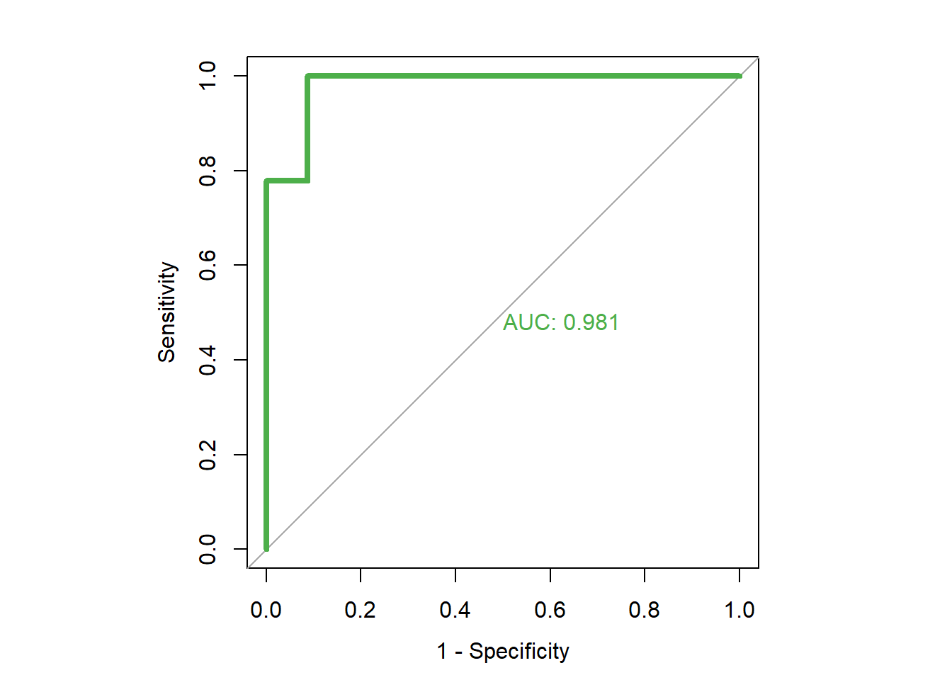
##
## Call:
## roc.default(response = dfinal$high.mpg, predictor = dfinal$rf.prob,     plot = TRUE, legacy.axes = TRUE, col = "#4daf4a", lwd = 4,     print.auc = TRUE)
##
## Data: dfinal$rf.prob in 23 controls (dfinal$high.mpg 0) < 9 cases (dfinal$high.mpg 1).
## Area under the curve: 0.9807
Above, we began with the command par(pty = "s"), which resets the plot dimensions So that our ROC curve will be formatted nicely.
We then use the roc function with the following arguments:
dfinal$high.mpg– These are the true classes that we are trying to predict.dfinal$rf.prob– These are the predicted probabilities that each observation will be in the high class (coded as1inhigh.mpg).plot=TRUE– This tells the computer to give us a visual plot, in addition to the numeric output with summary statistics.legacy.axes=TRUE– This tells the computer to use axes for the plot that are consistent with traditional conventions.col="#4daf4a"– This tells the computer the color to use when drawing the curve.lwd=4– This tells the computer how thick to make the curve that is plotted.print.auc=TRUE– This tells the computer to print the AUC—area under the curve—within the plot itself.
As you can see from the output, the AUC is very high for this model. It is very close to 1, which is the maximum possible value.
12.4.2 ROC for linear regression
Now we will repeat the very same procedure for our linear regression results, which we can find in the saved dataset dfinal2. I will repeat the procedure below but without much narration or commentary..
Calculate probabilities:
dfinal2$lm.prob <- dfinal2$lm.pred/max(dfinal2$lm.pred)Make ROC curve:
par(pty = "s")
roc(dfinal2$high.mpg, dfinal2$lm.prob, plot=TRUE, legacy.axes=TRUE, col="#377eb8", lwd=4, print.auc=TRUE)
## Setting levels: control = 0, case = 1## Setting direction: controls < cases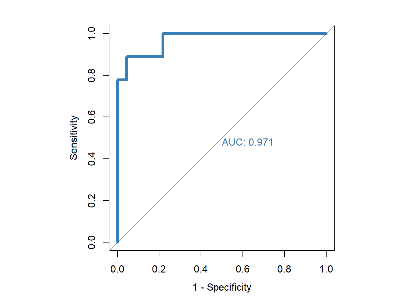
##
## Call:
## roc.default(response = dfinal2$high.mpg, predictor = dfinal2$lm.prob,     plot = TRUE, legacy.axes = TRUE, col = "#377eb8", lwd = 4,     print.auc = TRUE)
##
## Data: dfinal2$lm.prob in 23 controls (dfinal2$high.mpg 0) < 9 cases (dfinal2$high.mpg 1).
## Area under the curve: 0.971
Above, for our linear regression results, we see an AUC that is still very high but somewhat lower than that of the random forest model.
12.4.3 Combined ROC plot
Now that we have individually creative ROC curves for the two cross-validated predictive models that we ran earlier, we can plot these curves against each other on a single plot. I find it easiest to give this command all at once, in a single R markdown code chunk:
par(pty = "s")
roc(dfinal$high.mpg, dfinal$rf.prob, plot=TRUE, legacy.axes=TRUE, col="#4daf4a", lwd=4, print.auc=TRUE)

plot.roc(dfinal2$high.mpg, dfinal2$lm.prob, legacy.axes=TRUE, col="#377eb8", lwd=4, print.auc=TRUE, add=TRUE, print.auc.y=.4)

legend("bottomright", legend=c("Random Forest", "Linear Regression"), col=c("#4daf4a", "#377eb8"), lwd=4)
Above, you can see the entire code chunk to create the combined ROC plot. Below, you will see parts of the chunk above as they are executed. First, we run the par and roc commands just like we did to make the single ROC curve for the random forest results. Then, we add the ploc.roc and legend commands which add the ROC curve or the linear regression results to the same plot, so that we can view them against each other. I will explain the details of the plot.roc command below, after you see the results.
par(pty = "s")
roc(dfinal$high.mpg, dfinal$rf.prob, plot=TRUE, legacy.axes=TRUE, col="#4daf4a", lwd=4, print.auc=TRUE)
##
## Call:
## roc.default(response = dfinal$high.mpg, predictor = dfinal$rf.prob, plot = TRUE, legacy.axes = TRUE, col = "#4daf4a", lwd = 4, print.auc = TRUE)
##
## Data: dfinal$rf.prob in 23 controls (dfinal$high.mpg 0) < 9 cases (dfinal$high.mpg 1).
## Area under the curve: 0.9807plot.roc(dfinal2$high.mpg, dfinal2$lm.prob, legacy.axes=TRUE, col="#377eb8", lwd=4, print.auc=TRUE, add=TRUE, print.auc.y=.4)
legend("bottomright", legend=c("Random Forest", "Linear Regression"), col=c("#4daf4a", "#377eb8"), lwd=4)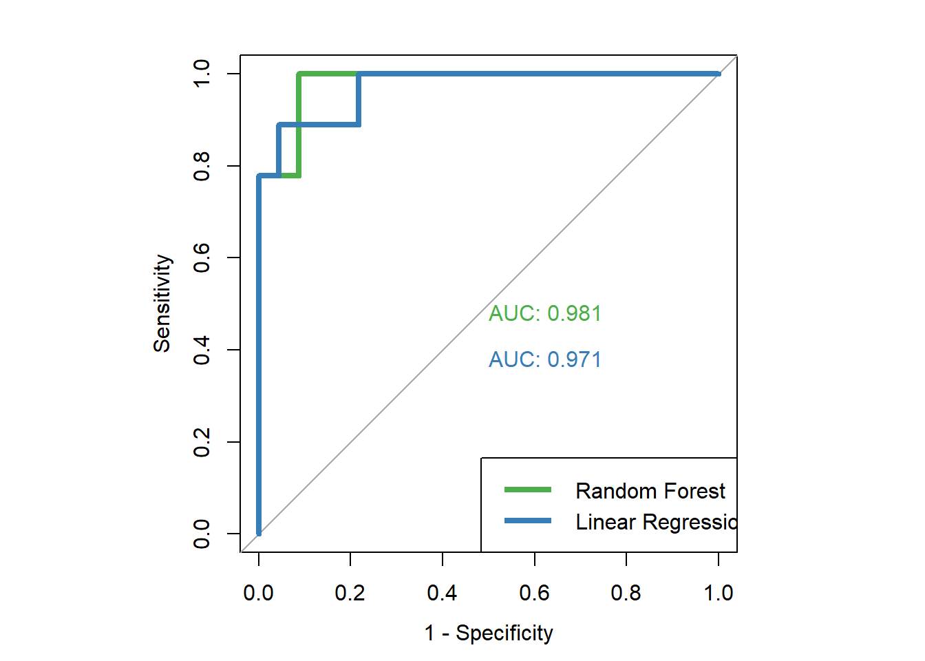
Let’s go through the plot.roc command’s arguments:
dfinal2$high.mpg, dfinal2$lm.prob, legacy.axes=TRUE, col="#377eb8", lwd=4, print.auc=TRUE– All of these arguments are the same as when we used theroc(...)command a little while ago, in this section of the chapter, while making the separate ROC curves for each model’s results.add=TRUE– This tells the computer to add the ROC curve for the linear regression result (lm.prob) to the already-plotted plot for the ROC curve for the random forest result (rather than making a separate plot).print.auc.y=.4– This tells the computer where in the plot to position the AUC metric readout for the second ROC curve, so that it doesn’t overlap with the AUC readout from the first ROC curve.
And now we’ll go through the legend command’s arguments:
"bottomright"– This tells the computer that we want the legend to go to the bottom-right corner of the plot.legend=c("Random Forest", "Linear Regression")– This programs the plot’s legend such that the first curve is labeled as random forest and the second one is labeled as linear regression.col=c("#4daf4a", "#377eb8")– This assigns colors to each line.lwd=4– This determines the thickness of the lines.
Now that we are done making our ROC curves and plotting them, let’s reset the formatting option that we had changed earlier with the par command:
par(pty = "m")Now the settings have been changed back to how they were originally.
12.4.4 ROC curves wrap-up
Above, we learned how to make ROC curves for predictive models on which we had already calculated predictions. More specifically, we used the known true classifications (high or low miles per gallon) as well as predicted probabilities of testing data having high miles per gallon. With these two pieces of information for all of our observations, we are able to make ROC curves in R. Additionally, we can put these curves on the same plot as each other to compare the predictive capability of the various models against each other.
12.5 Confusion matrix metrics
In this final part of the chapter, we will review some metrics that are used to determine how useful a predictive model is. All of these metrics are ones that you have already read about or used in other assignments/chapters, but we have not reviewed how to easily calculate these in R.
Optional review reading:
- Agarwal R. (17 Sep 2019). The 5 Classification Evaluation metrics every Data Scientist must know. (https://towardsdatascience.com/the-5-classification-evaluation-metrics-you-must-know-aa97784ff226){target=“_blank”}.
We will use the caret package to calculate the metrics we want. So we will begin by loading the package:
if(!require(caret)) install.packages('caret')
library(caret)
The confusionMatrix function within caret is a useful command that you can use frequently. Here is how the arguments of this command work:
caret::confusionMatrix(PredictedValues, ActualValues)When you use the command above, the first argument should be the predicted values calculated by the model you created, and the second argument should be the actual true values. We will follow this approach below when we use the confusionMatrix command on the predictive models that we ran earlier.
12.5.1 Random forest metrics
Now we will calculate some metrics for our random forest model:
cm.rf <- caret::confusionMatrix(as.factor(dfinal$rf1.pred.high), as.factor(dfinal$high.mpg))Above, we used the confusionMatrix function in the caret package to create and store a confusion matrix called cm.rf. To create cm.rf, we used the discretized random forest predictions from dfinal and the discretized true mpg values from dfinal. When we first created these variables, they were coded as numeric variables, even though they only have two values (1 and 0). The confusionMatrix function requires it’s arguments to be factor variables. So we have converted the variables two factors using the as.factor(...) function in the code above.
Now that we have created cm.rf, the caret package will do the rest of the work for us and calculate the metrics we want. First, we can simply inspect the confusion matrix that we just saved:
cm.rf## Confusion Matrix and Statistics
##
## Reference
## Prediction 0 1
## 0 21 0
## 1 2 9
##
## Accuracy :
## 95% CI :
## No Information Rate :
## P-Value [Acc > NIR] :
##
## Kappa :
##
## Mcnemar's Test P-Value :
##
## Sensitivity :
## Specificity :
## Pos Pred Value :
## Neg Pred Value :
## Prevalence :
## Detection Rate :
## Detection Prevalence :
## Balanced Accuracy :
##
## 'Positive' Class :
##
##
## 0.9375
## (0.7919, 0.9923)
## 0.7188
## 0.002302
##
## 0.8552
##
## 0.479500
##
## 0.9130
## 1.0000
## 1.0000
## 0.8182
## 0.7188
## 0.6562
## 0.6562
## 0.9565
##
## 0
## In the output above, the two by two confusion matrix is shown at the top and then a huge variety of metrics are given below, for that confusion matrix. This is an easy way to quickly assess the results of your predictive classification. Note that Reference refers to actual true values of the dependent variable and Prediction refers to the predicted values from the machine learning model (assuming you input them correctly into the computer).
You can get additional information with the command below:
cm.rf$byClass## Sensitivity Specificity
## 0.9130435 1.0000000
## Pos Pred Value Neg Pred Value
## 1.0000000 0.8181818
## Precision Recall
## 1.0000000 0.9130435
## F1 Prevalence
## 0.9545455 0.7187500
## Detection Rate Detection Prevalence
## 0.6562500 0.6562500
## Balanced Accuracy
## 0.9565217Keep in mind that…
- Sensitivity and recall are the same.
- Positive predictive value and precision are the same.
12.5.2 Linear regression metrics
Above, we created a confusion matrix and looked at its metrics for our random forest model. Below, we will do the same for our linear regression model:
cm.lm <- caret::confusionMatrix(as.factor(dfinal2$reg1.pred.high), as.factor(dfinal2$high.mpg))cm.lm## Confusion Matrix and Statistics
##
## Reference
## Prediction 0 1
## 0 18 0
## 1 5 9
##
## Accuracy :
## 95% CI :
## No Information Rate :
## P-Value [Acc > NIR] :
##
## Kappa :
##
## Mcnemar's Test P-Value :
##
## Sensitivity :
## Specificity :
## Pos Pred Value :
## Neg Pred Value :
## Prevalence :
## Detection Rate :
## Detection Prevalence :
## Balanced Accuracy :
##
## 'Positive' Class :
##
##
## 0.8438
## (0.6721, 0.9472)
## 0.7188
## 0.07919
##
## 0.6694
##
## 0.07364
##
## 0.7826
## 1.0000
## 1.0000
## 0.6429
## 0.7188
## 0.5625
## 0.5625
## 0.8913
##
## 0
## cm.lm$byClass## Sensitivity Specificity
## 0.7826087 1.0000000
## Pos Pred Value Neg Pred Value
## 1.0000000 0.6428571
## Precision Recall
## 1.0000000 0.7826087
## F1 Prevalence
## 0.8780488 0.7187500
## Detection Rate Detection Prevalence
## 0.5625000 0.5625000
## Balanced Accuracy
## 0.8913043As you can see above, we once again get the same metrics for the linear regression model confusion matrix that we got for the random forest model confusion matrix.
12.6 Assignment
In this week’s assignment, you will use a dataset of your own choosing to practice the techniques demonstrated in this chapter. It will save you time if you use the same data that you used for the Chapters 8 and/or 10 assignment on regression and classification. To do this assignment, I recommend that you choose your two favorite predictive models from your Chapters 8 and 10 assignment and re-use those for this Chapter 12 assignment below. It is fine to choose either regression or classification models to use in this assignment; both will work equally well. If you follow this recommendation, you will be taking your two best models from Chapter 8 or 10’s assignments and you will just be evaluating the results in new ways.50
For example, let’s say that you have a categorical dependent variable and your best results so far came from a logistic regression model in week 8 and a KNN classification model in week 10. In this case, you can simply use these two types of models in the week 12 assignment below. Or you can choose two models that are both from Chapter 10. It’s up to you. If you have a numeric dependent variable, you can choose your favorite two models from your linear regression results in week 8 and the three models you ran in week 10 (KNN regression, regression tree, random forest regression).
In the examples given in this chapter, the predictive models created were all made using a continuous numeric dependent variable, and therefore they use regression techniques instead of classification techniques. However, everything demonstrated earlier in this chapter can also be done using classification techniques. To use a classification technique (instead of a regression technique) in your cross-validated model, simply replace the following line in your for loop with whichever type of predictive model you want to create:
rf1 <- randomForest(mpg ~ .,data=dtrain, proximity=TRUE,ntree=1000)
Above, you could write the code for a logistic regression model or random forest classification model, for example, and the cross-validation process would still work.51 All that matters is that you are using the correct training and testing data sets. You should not modify the research question you are asking just to do cross-validation. You can use a binary or numeric dependent variable, whichever you prefer. The procedure you follow will be the same in either case. Feel free to ask for help related to this.
12.6.1 Cross-validation
You will begin this assignment by practicing cross-validation. For the most part, you should be able to take and modify the code that was used earlier in this chapter. Then you will compare the results of the models you make to each other using selected metrics.
Task 1: Briefly provide the research question, dependent variable, and number of observations for the data that you plan to use for this assignment.
Task 2: Create cross-validated models using at least two prediction techniques and store the results, as is demonstrated earlier in this chapter. You can choose from linear/logistic regression, KNN, random forest, or any other predictive methods that you think are reasonable, as long as you use two different methods and you use cross-validation. Remember that it’s completely fine to do either classification or regression.
Task 3: For both cross-validated model results, present a scatterplot with actual and predicted values plotted against each other. If you have a binary dependent variable, this scatterplot is unlikely to be meaningful, but it is good to still practice making it.
Task 4: Present confusion matrices to show your two results.52 Use the confusionMatrix function in the caret package to present the matrices.
Task 5: By hand, calculate precision and recall for both of the confusion matrices you made. Show your calculations. Do they match the values of precision and recall given by the caret package? If not, you might need to reverse the positions of the actual and predicted values in the caret::confusionMatrix(...) function.
Task 6: By hand, calculate sensitivity and specificity for both of the confusion matrices you made. Show your calculations. Do they match the values of sensitivity and specificity given by the caret package? If not, you might need to reverse the positions of the actual and predicted values in the caret::confusionMatrix(...) function.
Task 7: Interpret the accuracy, specificity, sensitivity, precision, and recall for the two predictive results. Is one model clearly better than the other? Is there a trade-off between the two? Is neither model good? Which metrics helped you determine this, and why?
12.6.2 ROC curves
Following the lead of the demonstration in this chapter, you will now use ROC curves to compare the two predictive models that you made earlier with cross-validation.
Task 8: Create a single plot showing the ROC curves for both of the cross-validated predictive models that you made earlier in this assignment. This plot should also have a correctly labeled legend and should display the AUC for each curve.
Task 9: Compare the two ROC curves. Which model is better? How do you know this from looking at the ROC curve?
Task 10: Compare the AUC for the two curves. Which one has the better AUC? Is it the model that you expected to be better?
12.6.3 Follow-up and submission
You have now reached the end of this week’s assignment. The tasks below will guide you through submission of the assignment and allow us to gather questions and feedback from you.
Task 11: Please write any questions you have this week (optional).
Task 12: Write any feedback you have about this week’s content/assignment or anything else at all (optional).
Task 13: Submit your final version of this assignment to the appropriate assignment drop-box in D2L.
Note that the k in k-fold cross-validation is different than the k in the k-nearest neighbors machine learning algorithm.↩︎
You can try this out for yourself. Type the following code into the console in R and see the output:
cat("Hello","my","name","is"↩︎Calculating predicted probabilities using a different technique would also be acceptable or even better in some situations. For example, predicted probabilities taken directly from a random forest or logistic regression model could be used, in situations where the dependent variable is categorical and you are doing classification instead of regression.↩︎
Note that it is NOT a requirement that you re-use models from Chapters 8 or 10; it is also fine for you to use new data and models in your Chapter 12 if you prefer, but it might be more time consuming. One good reason for NOT re-using your Chapters 8 and 10 predictive models is if you are doing a final project that involves data analysis and you did not use your final project data in Chapters 8 or 10, but now you are ready to use it in Chapter 12. Using final project data for Chapter 12 will still make it easier for you to complete your final project in this class.↩︎
Note that to run a cross-validated KNN model, you will need to replace the random forest line of code with multiple new lines of code, not just a single new line. All all it will still be done within the for loop.↩︎
If you used a numeric dependent variable, you will first have to decide how to discretize your actual and predicted values before you make the confusion matrix. You can additionally—but not as a substitute—calculate the RMSE if you would like.↩︎