Chapter 8 Regression methods for supervised machine learning in R
8.1 Goals and introduction
This week, our goals are to…
Split data into testing and training sets for use with regression.
Use regression analysis to make predictions.
In this chapter, we will use supervised machine learning to use basic linear and logistic regression models to make predictions. You have the option of using the student-por.csv data in your assignment this week if you would like, but I also encourage you to use your own data if you have some. We are also available to meet with you to look at your data and/or assist with preparing it for use in predictive analysis.
The following tutorial shows how to import, split (into training and testing), and create a model with your data. Then, we will look at how to use the models to make predictions and measure how good or bad the model is at making predictions for us.
We will be using supervised machine learning in this tutorial, which means that we must look at a dependent variable that is an outcome of interest. In other words, there should be a variable in the data that it would be useful to us to be able to predict in advance. In the case of this example tutorial, we will treat the variable mpg from within the mtcars dataset as our dependent variable of interest.
8.2 Import and prepare data
This part of our procedure is very similar to how we imported and prepared data in earlier portions of this course.
For the examples in this tutorial, I will again just use the mtcars dataset that is already built into R. However, we will still “import” this and give it a new name—df—so that it is easier to type.
df <- mtcarsRun the following command in your own R console to see information about the data:
?mtcarsAnd we can see all of the variable names, like we have done before:
names(df)## [1] "mpg" "cyl" "disp" "hp" "drat" "wt" "qsec" "vs" "am"
## [10] "gear" "carb"Number of observations:
nrow(df)## [1] 32Remove missing observations:
df <- na.omit(df)Inspect some rows in the dataset:
head(df)## mpg cyl disp hp drat wt qsec vs am gear
## Mazda RX4 21.0 6 160 110 3.90 2.620 16.46 0 1 4
## Mazda RX4 Wag 21.0 6 160 110 3.90 2.875 17.02 0 1 4
## Datsun 710 22.8 4 108 93 3.85 2.320 18.61 1 1 4
## Hornet 4 Drive 21.4 6 258 110 3.08 3.215 19.44 1 0 3
## Hornet Sportabout 18.7 8 360 175 3.15 3.440 17.02 0 0 3
## Valiant 18.1 6 225 105 2.76 3.460 20.22 1 0 3
## carb
## Mazda RX4 4
## Mazda RX4 Wag 4
## Datsun 710 1
## Hornet 4 Drive 1
## Hornet Sportabout 2
## Valiant 1In other instances, we would have scaled or standardized our data. It is not necessary for us to do this when using linear or logistic regression.
8.3 Linear regression to make predictions
This portion of the tutorial will demonstrate how to use linear regression to make predictions. You will then repeat this process with different data and some additional modifications in your assignment for the week.
Our goal in this portion of the tutorial is to predict each car’s mpg as accurately as possible.
8.3.1 Divide data
Now that our data is ready, we will start our analysis by dividing the data into testing and training datasets. The training data will be used to create a new predictive model. The testing data—which was not used to create the model and which will be new to the computer—will be plugged into the model to see how well the model makes predictions.
Below, you’ll find the code we use to split up our data. For now, I have decided to use 75% of the data to train and 25% of the data to test. Here’s the first line of code to start the splitting process:
trainingRowIndex <- sample(1:nrow(df), 0.75*nrow(df)) # row indices for training dataThe code above does the following:
- Figure out the number of observations in the dataset
df. If you’re using a different dataset, changedfto the name of your own data when you use this code. - Randomly select 75% of the rows in
df. You can change the0.75written in the code if you want to change the proportion of training and testing data.
Above, we randomly selected the rows that we would be including in each dataset, but we didn’t actually create the new datasets. So let’s start by creating the training data:
dtrain <- df[trainingRowIndex, ] # model training dataAbove, we created a new dataset called dtrain which contains the 75% of observations which were selected for inclusion in the training dataset.
And now we’ll create the testing dataset:
dtest <- df[-trainingRowIndex, ] # test dataAbove, we created a new dataset called dtest which contains the remaining 25% of observations which are not part of the training dataset.
So we now have three datasets:
df– This is the original full dataset. We won’t use this much for the rest of the tutorial, but we could refer to it if we need to.dtrain– A training dataset containing 75% of the observations.dtest– A testing dataset containing 25% of the observations.
We can verify if our data splitting procedure worked:
nrow(dtrain)## [1] 24nrow(dtest)## [1] 8Above, we see that the training data contains 24 observations and the testing data contains 8 observations.
You can also look at these two datasets by running the following commands, one at a time, in your console (not your RMarkdown or R code file):
View(dtrain)
View(dtest)
Running the commands above will open a spreadsheet viewer on your computer for you to look at the data. There’s no way to display that within a “knitted” RMarkdown document or in the textual results that we usually get from R. That’s why the View command should never be included in your RMarkdown code.
8.3.2 Run linear regression
We are now ready to make our first predictive model, an ordinary least squares (OLS) linear regression model. We will do this using the training data as follows:
reg <- lm(mpg ~ ., data = dtrain)The code above creates and stores the results of a new linear regression model. Here are the details:
- The name of the stored model is
reg. - The dependent variable is designated as
mpg. - All of the other variables in the dataset are designated as independent variables; that’s what the
~ .part of the code means. - We could also write the name of each IV (independent variable) instead, if we wanted to just select a subset of them, like this:
mpg ~ IV1 + IV2 + IV3and so on. - We specified at the end of the command that we wanted to use the
dtraindata to make this regression model.
Now that we have created and stored the results of a regression model, we can use it to make predictions for us on our data.
8.3.3 Make predictions
Below is the key line of code that you will use to plug new data into a preexisting stored model. In this case, our new data on which we want to make predictions is called dtest. Here it is:
dtest$reg.mpg.pred <- predict(reg, newdata = dtest)Above, we added a variable (column of data) to the dtest data. This new column is called reg.mpg.pred. This new variable stores all of the predicted values of mpg for the testing data. To calculate this prediction, for each row of the test data, the computer plugged the values of the independent variables into the stored regression model reg. Plugging in those independent variables gave the computer a prediction for the dependent variable in that row. This value was then saved as reg.mpg.pred for that row.
The computer knew that this is what we wanted to do because we specified in the predict function that we wanted to make predictions using the stored reg model and we wanted to plug dtest into that model as fresh data.
Now that we have made our predictions, we can see how good they are!
8.3.4 Check accuracy
This section demonstrates a few selected ways to test accuracy of a regression model.
8.3.4.1 Actual and predicted values
First, since our dataset is not that large, let’s start by simply looking at the true and predicted values of mpg for the testing data side by side. Remember, we care the most about how the model performs on the testing data, because our goal is to use this model to make predictions on new data in the future.
Here is the code and result that shows us the true values of mpg and the predicted values of mpg for eight cars for which we made predictions (because these were the cars that were randomly split into the testing dataset, which were not used to train the model):
dtest[c("mpg","reg.mpg.pred")]## mpg reg.mpg.pred
## Hornet 4 Drive 21.4 21.36493
## Duster 360 14.3 15.51104
## Merc 230 22.8 32.26509
## Merc 280C 17.8 20.47901
## Toyota Corona 21.5 29.01088
## Pontiac Firebird 19.2 15.16593
## Fiat X1-9 27.3 29.15442
## Volvo 142E 21.4 26.00033Above, we see, for example, that the car Pontiac Firebird truly has an mpg of 19.2 and the model predicted that it would have an mpg of 15.2. So the prediction is off by 4 units. Whether that much error is acceptable or not is up to you, the user of the predictive model. There is no right or wrong answer necessarily.
We can also look at the data from the table above as a scatterplot:
plot(dtest$reg.mpg.pred,dtest$mpg)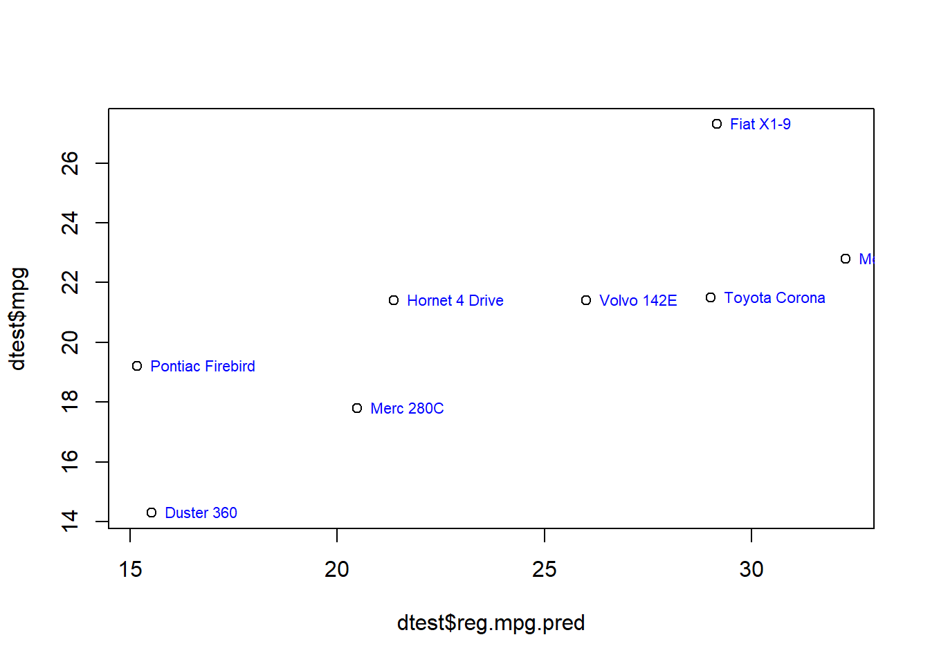
The plot above has shows the true mpg values for each car on the vertical axis (y-axis) and the model’s predicted values for each car’s mpg on the horizontal axis (x-axis). It shows 8 plotted points (circular dots), one for each car in the testing dataset.
When we look at the plot, it shows that there is an overall positive trend, meaning that overall the predictions increase as the true values increase, but there is also a lot of error. If there were no errors, the dots would all be on a straight line and every actual value would be the same as very predicted value. You can locate the Pontiac Firebird on this graph. It’s the dot that is in between 18 and 20 on the vertical axis towards the very bottom. It is at approximately 15 on the horizontal axis.
We can also re-plot this and include the labels of each car in the plot:
plot(dtest$reg.mpg.pred,dtest$mpg)
text(dtest$reg.mpg.pred,dtest$mpg, row.names(dtest), cex=0.7, pos=4, col="blue")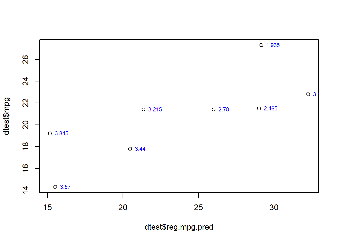
If we want, we can label each point with any variable from the dataset. Below, we’ll label each point with each car’s weight, which is the variable wt.
plot(dtest$reg.mpg.pred,dtest$mpg)
text(dtest$reg.mpg.pred,dtest$mpg, dtest$wt, cex=0.7, pos=4, col="blue")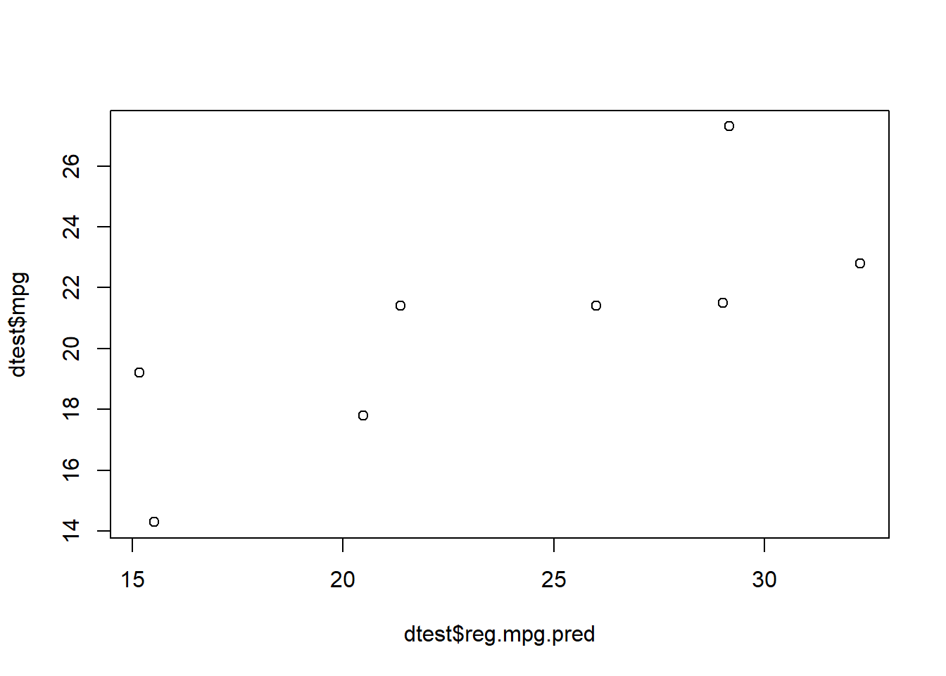
Next, we’ll look at another key measurement that is often used when predicting numeric outcomes in predictive analytics.
8.3.4.2 RMSE
RMSE (root mean square error) is a very common metric that is used to calculate the accuracy of a predictive model when the dependent variable is a continuous numeric variable. This is considered to be better than other metrics—such as \(R^2\)—when measuring how useful a model is with fresh (testing) data.
If you wish, you can read more about RMSE here, but it is not required for you to do so:
Moody, J. (2019). What does RMSE really mean? https://towardsdatascience.com/what-does-rmse-really-mean-806b65f2e48e.
Let’s calculate the RMSE for the predictive model we just made. To do this, we use the rmse function from the Metrics package and we feed the actual and predicted values (which we calculated earlier) into the function:
if(!require(Metrics)) install.packages('Metrics')
library(Metrics)

rmse(dtest$mpg,dtest$reg.mpg.pred)
## [1] 4.943707Above, we see that the RMSE of this model on this particular testing data is 4.9. You will get a sense for good and bad values of RMSE as you use this metric more and more. Usually, it helps us compare predictive models to each other.
8.3.4.3 Discretize and check
Another way that we can check our model’s accuracy is to discretize the data. This means that we will sort the data into discrete categories. In this case, we will just sort the mpg data into high and low values of mpg. Let’s start off by saying that a car has high mpg if it has a value of mpg over 22. Let’s do this first for the true values of mpg in the testing data:
dtest$high.mpg <- ifelse(dtest$mpg>22,1,0)Above, we told the computer, to create a new discrete binary variable (meaning a variable with only two possible levels). The value of this variable will be 1 for all cars with mpg greater than 22 and 0 for all cars with mpg less than or equal to 22.
Below, we’ll do the same for the predicted values of mpg (which are saved as reg.mpg.pred):
dtest$high.mpg.pred <- ifelse(dtest$reg.mpg.pred>22,1,0)Above, the new variable high.mpg.pred was created (and added to dtest), which will also have values of 1 or 0 to indicate whether the predicted (not true/actual) value of mpg for each car is high or low, again using 22 as a cutoff threshold.
Let’s inspect our data again to look at what we just did, just to be clear:
dtest[c("mpg","high.mpg","reg.mpg.pred","high.mpg.pred")]## mpg high.mpg reg.mpg.pred high.mpg.pred
## Hornet 4 Drive 21.4 0 21.36493 0
## Duster 360 14.3 0 15.51104 0
## Merc 230 22.8 1 32.26509 1
## Merc 280C 17.8 0 20.47901 0
## Toyota Corona 21.5 0 29.01088 1
## Pontiac Firebird 19.2 0 15.16593 0
## Fiat X1-9 27.3 1 29.15442 1
## Volvo 142E 21.4 0 26.00033 1And again, you can inspect the entire dataset yourself by running the following command in the console:
View(dtest)Now that we have successfully discretized our data, we can make a confusion matrix that shows how many predictions were correct and incorrect:
with(dtest,table(high.mpg,high.mpg.pred))## high.mpg.pred
## high.mpg 0 1
## 0 4 2
## 1 0 2Every time we interpret the results of a confusion matrix like this one, we will write four key sentences. Here are these four key sentences for the confusion matrix above, which was generated using 22 as the cutoff between low (coded as 0) and high (coded as 1):
- 4 cars truly have low
mpgand were correctly predicted to have lowmpg. These are true negatives. - 0 cars that truly have high
mpgwere incorrectly predicted to have lowmpg. These are false negatives. - 2 cars that truly have low
mpgwere incorrectly predicted to have highmpg. These are false positives. - 2 cars that truly have high
mpgwere correctly predicted to have highmpg. These are true positives.
Above, we assumed that a low mpg is a good thing and a high mpg is bad. That’s why we labeled cars with low mpg as negatives and high mpg as positives.
Next, let’s change the threshold. Let’s keep the true meaning of high and low as 22. But let’s change the sensitivity and specificity of our predictions by modifying the threshold for the predicted values. First, we’ll lower it by 4 units, from 22 to 18. This will make our predictions more likely to classify cars as high mpg, because now all cars between 18 and 22 will also be included as high mpg, whereas before only cars above 22 were considered high mpg.
Here is the modified code which sets the prediction threshold at 18 and then creates a new confusion matrix:
dtest$high.mpg <- ifelse(dtest$mpg>22,1,0)
dtest$high.mpg.pred <- ifelse(dtest$reg.mpg.pred>18,1,0)
with(dtest,table(high.mpg,high.mpg.pred))
## high.mpg.pred
## high.mpg 0 1
## 0 2 4
## 1 0 2Above, out of the 6 cars in total that truly have low mpg, 2 were predicted correctly to have low mpg and 4 were predicted incorrectly to have high mpg. If you compare this to the confusion matrix from before (at the 22 threshold), two of these six cars jumped from low prediction to high prediction.
Let’s try this one more time. This time, we’ll make the threshold (only for the predictions) 4 points higher than 22:
dtest$high.mpg <- ifelse(dtest$mpg>22,1,0)
dtest$high.mpg.pred <- ifelse(dtest$reg.mpg.pred>26,1,0)
with(dtest,table(high.mpg,high.mpg.pred))
## high.mpg.pred
## high.mpg 0 1
## 0 4 2
## 1 0 2Above, we set the cutoff threshold to 26 for the predictions. We get the very same predictions that we got when we used 22. So the accuracy, sensitivity, and specificity are the same in both cases.
Which of these three prediction cutoff thresholds should you use when making predictions about new cars for which you do not know the true mpg? That is up to you. It largely depends on whether you want cars that the model is uncertain about to be classified as low or high mpg.
8.3.5 Variable importance
Using the varImp function from the caret package, as shown below, we can rank how important each independent variable was in helping us make a prediction in our linear regression:
if(!require(caret)) install.packages('caret')## Warning: package 'caret' was built under R version 4.2.3## Warning: package 'lattice' was built under R version 4.2.3library(caret)
varImp(reg)## Overall
## cyl 0.98346899
## disp 0.16693025
## hp 0.84666403
## drat 1.08329247
## wt 1.66379377
## qsec 1.62719740
## vs 0.76176942
## am 0.15662440
## gear 0.05210547
## carb 0.09612851Above, wt is considered to be the most useful variable in helping us make a prediction about mpg, because it has the highest number.
Later, if we wanted, we could try to make a predictive regression model using only the few most important variables as independent variables.
8.3.6 Linear regression wrap-up
So far, you have seen how linear regression is used to make predictions of a continuous numeric dependent variable (mpg) on individual observations (cars). You then saw how to check how useful those predictions are.
Next, we’ll repeat the same procedure using logistic regression.
8.4 Logistic regression to make predictions
Logistic regression helps us predict binary outcomes, which we can think of as yes-no or 1 or 0 outcomes. In our case, we want to predict if a car has high or low mpg, so this fits within our goal. This procedure will follow the same process you saw for linear regression, with a few differences.
8.4.1 Prepare and divide data
Let’s use the same training-testing division from before, so that we can easily compare results of the linear and logistic models to each other using the same testing cars. So again, we’ll use dtrain and dtest which are already stored in the computer for us to use.
Now that we are using logistic regression, our dependent variable has to be transformed into a yes or no variable. We will use 1 to mean yes and 0 to mean no. Below, we create a new variable called high.mpg which is yes if mpg is over 22 and no otherwise:33
dtrain$high.mpg <- ifelse(dtrain$mpg>22,1,0)Now our new variable high.mpg has been created and added to our dataset. This will be our dependent variable throughout the logistic regression section of this tutorial. We are no longer using the original mpg as the dependent variable. Therefore, we should remove mpg from our dataset before we continue:
dtrain$mpg <- NULLThe code above removed the variable mpg. Let’s verify this by looking at the variables that we have in our training and testing datasets:
names(dtrain)## [1] "cyl" "disp" "hp" "drat" "wt"
## [6] "qsec" "vs" "am" "gear" "carb"
## [11] "high.mpg"names(dtest)## [1] "mpg" "cyl" "disp" "hp"
## [5] "drat" "wt" "qsec" "vs"
## [9] "am" "gear" "carb" "reg.mpg.pred"
## [13] "high.mpg" "high.mpg.pred"In dtrain, we have the dependent variable high.mpg and the same independent variables as before.
In dtest, we see some of the leftover additional variables from before when we did linear regression, but that’s fine. It won’t mess up our predictions when we eventually plug the testing data into the new logistic regression model.
Important note: Usually, your dataset will already contain a categorical variable that you want to use as a dependent variable, so you will NOT have to create your categorical dependent variable based on a numeric variable the way we did above, when we convered mpg into high.mpg.
8.4.2 Run regression
We are now ready to create our logistic regression model!
logit <- glm(high.mpg ~ ., data = dtrain, family = "binomial")## Warning: glm.fit: fitted probabilities numerically 0 or 1 occurredAbove, we did the same thing we did when we were doing linear regression, with the following changes:
- The result is stored as
logitinstead ofreg. - The function used to make the regression model is called
glminstead of justlm. - Now the dependent variable is
high.mpginstead ofmpg. - We added the argument
family = "binomial", which tells the computer that we want a binary logistic regression.
Note that we did get an error message, but this is likely due to the small sample size we are using right now. When you repeat this procedure in your assignment, this should not be a problem. If you do happen to get an error message, it is fine for you to ignore it and proceed as if you did not.
Now that our logistic regression result is stored as logit, we can use it to make predictions on the testing data.
8.4.3 Make predictions
Like we did before, let’s use the all-important predict function to make predictions on the testing data:
dtest$logit.mpg.pred <- predict(logit, newdata=dtest , type = "response")Above, we created a new variable called logit.mpg.pred which stores the predicted probability that each testing car is high or low mpg.
8.4.4 Check accuracy
Below, you’ll see how we can make different confusion matrices to see how useful our predictive model is.
8.4.4.1 Actual and predicted values
Let’s start by inspecting the predicted probabilities that we just calculated:
dtest[c("high.mpg", "logit.mpg.pred")]## high.mpg logit.mpg.pred
## Hornet 4 Drive 0 1.357050e-07
## Duster 360 0 1.185287e-12
## Merc 230 1 1.000000e+00
## Merc 280C 0 2.220446e-16
## Toyota Corona 0 1.000000e+00
## Pontiac Firebird 0 2.220446e-16
## Fiat X1-9 1 1.000000e+00
## Volvo 142E 0 1.000000e+00Above, on the left, we see high.mpg which contains the true values of whether each testing car has high or low mpg. On the right side, we see logit.mpg.pred which contains the predicted probability that each car will have high or low mpg. There are two mistakes made by the computer: Toyota Corona and Volvo 142E. Both of these cars truly have low mpg but they were predicted to have high mpg.
We can also visualize this in a box-plot:
boxplot(dtest$logit.mpg.pred ~ dtest$high.mpg)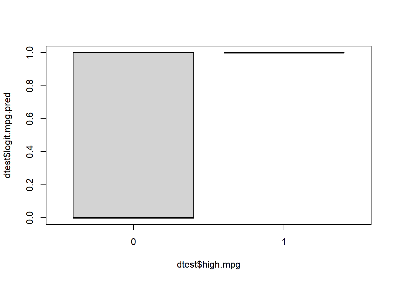
Above, we see that most but not all of the cars which truly have low mpg were correctly predicted to have low mpg. And all of the cars which truly have high mpg were correctly predicted to have high mpg.
8.4.4.2 Confusion matrix
Now we’ll turn back to confusion matrices. To make a confusion matrix, we have to decide which probability threshold we would like to use to classify a car as having high or low mpg. We’ll start with 0.5 as a cutoff and we will use the same coding approach that we did when discretizing our results with linear regression, earlier.
Here is the code to make a binary variable for our predictions, using the probabilities that we already have:
dtest$high.mpg.pred <- ifelse(dtest$logit.mpg.pred > 0.5, 1, 0)Now we have a new binary variable in our dtest data called high.mpg.pred. We can use it to make a confusion matrix:
with(dtest,table(high.mpg,high.mpg.pred))## high.mpg.pred
## high.mpg 0 1
## 0 4 2
## 1 0 2Here is our interpretation, again using the four key sentences for confusion matrix interpretation:
- 4 cars truly have low
mpgand were correctly predicted to have lowmpg. These are true negatives. - 2 cars truly have low
mpgbut were incorrectly predicted to have highmpg. These are false positives. - 0 cars truly have high
mpgbut were incorrectly predicted to have lowmpg. These are false negatives. - 2 cars truly have high
mpgand were correctly predicted to have highmpg. These are true positives.
Note that the order in which the sentences above are written does not matter.
Like before, we can change the cutoff threshold easily. Below, we change it to 0.75, keeping the rest of the code the same:
dtest$high.mpg.pred <- ifelse(dtest$logit.mpg.pred > 0.75, 1, 0)And again we create a confusion matrix:
with(dtest,table(high.mpg,high.mpg.pred))## high.mpg.pred
## high.mpg 0 1
## 0 4 2
## 1 0 2This time, the results happen to be exactly the same. But with more complicated and larger datasets, the results would potentially change when the threshold is adjusted.
8.4.5 Variable importance
Using the varImp function from the caret package, as shown below, we can rank how important each independent variable was in helping us make a prediction in our logistic regression:
if(!require(caret)) install.packages('caret')
library(caret)

varImp(logit)
## Overall
## cyl 1.560529e-05
## disp 3.024212e-06
## hp 1.096038e-05
## drat 1.607646e-05
## wt 1.792627e-06
## qsec 2.373447e-06
## vs 4.929542e-06
## am 7.151318e-06
## gear 1.279677e-06
## carb 6.282875e-06Above, am is considered to be the most useful variable in helping us make a prediction about mpg.
Later, if we wanted, we could try to make a predictive regression model using only the few most important variables as independent variables.
8.4.6 Logistic regression wrap-up
Above, you saw how to use binary logistic regression to make predictions of a binary (categorical) dependent variable (high.mpg) on individual observations (cars). You then saw how to check how useful those predictions are. This is an example of what we call classification, because cars were classified (sorted) into groups. It was never our goal to predict a continuous outcome. It was only our goal to sort observations into groups.
Next, we’ll briefly compare the linear and logistic regression results.
8.5 Compare linear and logistic predictions
Using a simple table, we can easily compare how well our linear and logistic regression models made predictions for us. We should also compare the confusion matrices that we created above to help us decide which model is best, especially if we had a larger dataset.
The stored dtest dataset has conveniently retained all of the data we need. Here’s the code:
dtest[c("mpg","reg.mpg.pred","high.mpg", "logit.mpg.pred")]## mpg reg.mpg.pred high.mpg logit.mpg.pred
## Hornet 4 Drive 21.4 21.36493 0 1.357050e-07
## Duster 360 14.3 15.51104 0 1.185287e-12
## Merc 230 22.8 32.26509 1 1.000000e+00
## Merc 280C 17.8 20.47901 0 2.220446e-16
## Toyota Corona 21.5 29.01088 0 1.000000e+00
## Pontiac Firebird 19.2 15.16593 0 2.220446e-16
## Fiat X1-9 27.3 29.15442 1 1.000000e+00
## Volvo 142E 21.4 26.00033 0 1.000000e+00Above, for example, we see that the Toyota Corona has a true value (mpg) of 21.5, which is a low value of high.mpg. The linear regression predicted this number to be 29.0. And the logistic regression predicted it to have a probability of nearly 0 of having a high mpg. So in this case, the logistic regression model correctly classified the Toyota Corona as having low mpg. But the linear regression model made a prediction for the Toyota Corona (29) which is much higher than the true value (21.5).
Again, it is up to you to decide which model would be best for your purposes for the situation in which you make predictions on brand new cars (for which the mpg is not known). It might also be the case that you decide not to use either of this models to make predictions in the future.
8.6 Assignment
In this week’s assignment, you are required to answer all of the questions below, which relate to using linear and logistic regression to conduct supervised machine learning. Please show R code and R output for all questions that require you to do anything in R. It is recommended that you submit this assignment as an HTML, Word, or PDF file that is “knitted” through RStudio.
If you have data of your own, it is strongly recommended that you use it this week instead of the provided data for this assignment. You can also request a meeting with an instructor to help you prepare your data or provide any other assistance that might be useful.
If you do want to use provided data, you should again use the student-por.csv dataset that we have used before. This is in D2L, if you don’t already have it downloaded. You can also get it from here:
- UCI Machine Learning Repository. Center for Machine Learning and Intelligent Systems. https://archive.ics.uci.edu/ml/datasets/Student+Performance. Download the file student.zip. Then open the file student-por.csv to see the data; this is the file you should load into R.
Here’s how you can load the data into R:34
df <- read.csv("student-por.csv")If you are using the student-por.csv, it is likely that no preprocessing steps will be necessary for you to do before you begin the analysis. If you are using your own data, you should conduct any preprocessing steps that you think are necessary before you start this assignment.
Important notes:
In this assignment, you will have the computer randomly split your data into training and testing datasets. Every time you do this, a new random split of the data will occur. This means that your results will be different every time, including when you Knit your assignment to submit it. As a result, the numbers in your written explanations will not match the numbers in your computer-generated outputs. This is completely fine. Please just write your answers based on the numbers you get initially and then submit your assignment even with the incorrect numbers that are generated when you Knit.
If you have a numeric dependent variable, use it for linear regression. Then, for logistic regression, “discretize” your numeric dependent variable into a binary variable and delete the original numeric variable from your dataset. If you have a binary dependent variable, use that binary dependent variable for both linear regression and logistic regression (you can ignore the fact that linear regression is not designed for binary dependent variables).
8.6.1 Prepare and divide data
In this first part of the assignment, you will prepare the data for further analysis.
Task 1: Divide your data into training and testing datasets.
Task 2: Double-check to make sure that you divided your data correctly and fix any errors.
Task 3: Specify a dependent variable of interest. This should be a continuous numeric variable.35 Use the variable G3 as your dependent variable if you are using the provided student-por.csv data.
Task 4: Write out the research question that your predictive analysis will help you answer and why that answer might be useful to know. Make sure that this is written as a “predictive analytics” research question rather than a “traditional statistics” research question.
8.6.2 Linear regression
Now you will use linear regression to make predictions.
Keep in mind that at any point, if you would like to produce a list of all variables in your dataset such that they are separated by a + and can easily be pasted into a regression formula, you can run the following code:
(b <- paste(names(d), collapse="+"))Then just copy-paste the resulting output and modify it as you see fit. It is a convenient way to avoid typing out all of your variable names. You can run the command
bagain any time you want, to recall the list of variables. You can delete the variables that you don’t want, after doing the copy-paste.
Task 5: Train a linear regression model to predict your dependent variable of interest.
Task 6: Make predictions on your testing data.
Task 7: Make a scatterplot showing actual and predicted values (for the testing data).
Task 8: Show a confusion matrix that you created using a selected cutoff threshold. Please provide an interpretation of the confusion matrix.
Task 9: Make a second confusion matrix showing predictions made at a different cutoff threshold. Please provide an interpretation of the confusion matrix. You can make as many confusion matrices as you would like.
Task 10: Manually36 calculate the accuracy of at least one of your models, based on the confusion matrix.
Task 11: Manually calculate the specificity of the same confusion matrix.
Task 12: Manually calculate the sensitivity of the same confusion matrix.
Task 13: How did the accuracy, sensitivity, and specificity change as you changed the cutoff threshold used to make the confusion matrix? You do not need to give the exact numbers when you answer this.
Task 14: Which metric—selecting from accuracy, sensitivity, and specificity—is most important for answering this particular predictive question?
Task 15: Create a ranking of variable importance for this model. Do the most important variables make sense to you as the most important ones?
Task 16: Modify the linear regression model you have been using such that there are fewer variables used to make the prediction (if you want, you can refer to the variable importance ranking when you do this). Train this new model and then test it again using the same procedure we used above, using a scatterplot, confusion matrices, accuracy, sensitivity, and specificity. To accomplish this task, you can simply make a copy of your code and slightly modify it. Please re-use the exact same training-testing data split that you used earlier, which means that you should NOT repeate the data splitting step from earlier.
Task 17: Calculate and compare the RMSE of your two linear regression models (calculated only on the testing data, of course).
8.6.3 Logistic regression
Turning to logistic regression, you will repeat the process above using a dependent variable that is already binary or by creating a binary variable out of the same continuous variable that you used above for linear regression. Once you create your new binary dependent variable, be sure to remove the original continuous numeric dependent variable from your dataset. We would not want it to be accidentally included as an independent variable.
Task 18: Create a logistic regression model to predict your dependent variable of interest.
Task 19: Make predictions on your testing data and show a confusion matrix that you created using a selected probability cutoff threshold. Please provide an interpretation of the confusion matrix.
Task 20: Make a second confusion matrix showing predictions made at a different cutoff threshold. You can make as many confusion matrices as you would like, each with different cutoff thresholds. Please provide an interpretation of the confusion matrix.
Task 21: Manually calculate the accuracy of at least one of your models, based on the confusion matrix.
Task 22: Manually calculate the specificity of the same confusion matrix.
Task 23: Manually calculate the sensitivity of the same confusion matrix.
Task 24: How did the accuracy, sensitivity, and specificity change as you changed the cutoff threshold used to make the confusion matrix? You do not need to give the exact numbers when you answer this.
Task 25: Which metric—selecting from accuracy, sensitivity, and specificity—is most important for answering this particular predictive question?
Task 26: Create a ranking of variable importance for this model. Do the most important variables make sense to you as the most important ones?
Task 27: Modify the logistic regression model you have been using such that there are fewer variables used to make the prediction (if you want, you can refer to the variable importance ranking when you do this). Train this new model and then test it again using the same procedure we used above (make a few confusion matrices at different cutoffs). Compare the initial and new models, in 2–4 sentences.
8.6.4 Compare models and make new predictions
Now we’ll practice choosing a predictive model that is best for our data.
Task 28: Compare the linear and logistic regression results that you just created. Would you prefer linear or logistic regression for making predictions on your dependent variable (on fresh data)? Be sure to explain why you made this choice, including the metrics and numbers you used.
Task 29: Using your favorite model that you already created, make predictions for your dependent variable on new data, for which the dependent variable is unknown. Present the results in a confusion matrix. This confusion matrix will of course only contain predicted values, because the actual values are not known. If you are using the student-por.csv data, you can click here to download the new data file called student-por-newfake.csv and make predictions on it. If you are using data of your own, you can a) use real new data that you have, b) make fake data to practice, or c) ask for suggestions. The true value of the dependent variable for the new data must be UNKNOWN.
8.6.5 Follow-up and submission
You have now reached the end of this week’s assignment. The tasks below will guide you through submission of the assignment and allow us to gather questions and feedback from you.
Task 30: Please write any questions you have this week (optional).
Task 31: Write any feedback you have about this week’s content/assignment or anything else at all (optional).
Task 32: Submit your final version of this assignment to the appropriate assignment drop-box in D2L.
Task 33: Don’t forget to do 15 flashcards for this week in the Adaptive Learner App at https://educ-app-2.vercel.app/.
I know we already did this earlier in our linear regression code, but this step is so important that I want to demonstrate it again, in this new context.↩︎
Of course, make sure you have properly set your working directory first!↩︎
Alternatively, you can specify two different dependent variables: one for use with linear regression and another for use with logistic regression.↩︎
Write out the formula for the calculation yourself and then plug in in the appropriate values and find the answer.↩︎