Chapter 4 Jun 5–11: Preprocessing and visualization
This week, our goals are to…
Apply basic procedures for data pre-processing and visualization in R.
Build competency in modifying code.
This week, please read this entire chapter and then complete the assignment at the end. While reading, you can follow along—if you would like—by copying the code from this chapter into your own RMarkdown file and running all of it in RStudio on your own computer (this is not required; it is just for extra). I also recommend that you quickly skim the assignment at the end of the chapter so that you are aware of what it asks you to do as you read this chapter.
4.1 Import data
4.1.1 Set working directory and import CSV file
Before we can proceed with pre-processing, we need to import our data into R. In your assignment, you will import the CSV file called student-por.csv (or you will use a dataset of your own choosing). The following procedure demonstrates how to import this data:
First, you need to set your working directory. This means that you need to tell R to “look” at the folder that contains the data you want to import. If you do not already know how to set the working directory, please refer to the section Set the working directory in R and RStudio at https://bookdown.org/anshul302/HE902-MGHIHP-Spring2020/jan-915-handling-data-in-r-linear-relationships-review.html#set-the-working-directory-in-r-and-rstudio.
Once the working directory is set, you can import the dataset:
d <- read.csv(file = "student-por.csv")After running the code above, the data from the file called student-por.csv is stored in R as the object d. We will refer to it as d in all of our R code. You can then do your analysis on the saved dataset d when it is time for you to do your assignment, at the end of this chapter.
If the code above does not work, please try the following code to load the student-por.csv dataset:
d <- read.csv(file = "student-por.csv", sep = ";")Above, we are telling the computer that the data in each cell of the data spreadsheet in each row of the csv file are separated by a semicolon character.
4.1.2 Prepare data for tutorial
4.1.2.1 Load data
The previous section demonstrates how to import the student-por.csv file that you might use in your homework assignment at the end of this chapter (unless you choose to use your own data). However, in the rest of this tutorial—before we get to the part where you do the assignment—we will use a different dataset. It is called 2015_16_Districtwise.csv and you can download it from https://www.kaggle.com/rajanand/education-in-india or find it in this week’s D2L section.
Here is a description of the dataset, from the link above:
Context: When India got independence from British in 1947 the literacy rate was 12.2% and as per the recent census 2011 it is 74.0%. Although it looks an accomplishment, still many people are there without access to education. It would be interesting to know the current status of the Indian education system. Content: This dataset contains district and state wise Indian primary and secondary school education data for 2015-16. Granularity: Annual.
The code below helps us import this data into R, once it has been downloaded to our computer:
d <- read.csv("2015_16_Districtwise.csv")Now we have a data frame12 loaded into R and it is called d. We could have chosen a different name instead of d, by changing the code above.13
We can explore how many observations (rows) are in the data:
nrow(d)## [1] 680Above, we see that there are 680 observations. In this case, each observation is a district in India. So, the unit of observation is the district.
Now let’s see how many variables (columns) are in the data:
ncol(d)## [1] 819Above we see that there are 819 variables. That’s a lot! It is very common for predictive analytics datasets to have a huge number of variables.
We can easily look at the row and columns by running a single command:
dim(d)## [1] 680 819As you can see above, the result of the dim() function gives us first the number of rows and then the number of columns.
We should now turn to more specific details about the variables. As a start, let’s see a list of all of the variables in the dataset:
names(d)## [1] "AC_YEAR" "STATCD"
## [3] "DISTCD" "STATNAME"
## [5] "DISTNAME" "DISTRICTS"
## [7] "BLOCKS" "VILLAGES"
## [9] "CLUSTERS" "TOTPOPULAT"
## [11] "P_URB_POP" "POPULATION_0_6"
## [13] "GROWTHRATE" "SEXRATIO"
## [15] "P_SC_POP" "P_ST_POP"
## [17] "OVERALL_LI" "FEMALE_LIT"
## [19] "MALE_LIT" "AREA_SQKM"
## [21] "TOT_6_10_15" "TOT_11_13_15"
## [23] "SCH1" "SCH2"
## [25] "SCH3" "SCH4"
## [27] "SCH5" "SCH6"
## [29] "SCH7" "SCH9"
## [31] "SCHTOT" "SCH1G"
## [33] "SCH2G" "SCH3G"
## [35] "SCH4G" "SCH5G"
## [37] "SCH6G" "SCH7G"
## [39] "SCH9G" "SCHTOTG"
## [41] "SCH1P" "SCH2P"
## [43] "SCH3P" "SCH4P"
## [45] "SCH5P" "SCH6P"
## [47] "SCH7P" "SCH9P"
## [49] "SCHTOTP" "SCH1M"
## [51] "SCH2M" "SCH3M"
## [53] "SCH4M" "SCH5M"
## [55] "SCH6M" "SCH7M"
## [57] "SCH9M" "SCHTOTM"
## [59] "SCH1GR" "SCH2GR"
## [61] "SCH3GR" "SCH4GR"
## [63] "SCH5GR" "SCH6GR"
## [65] "SCH7GR" "SCH9GR"
## [67] "SCHTOTGR" "SCH1GA"
## [69] "SCH2GA" "SCH3GA"
## [71] "SCH4GA" "SCH5GA"
## [73] "SCH6GA" "SCH7GA"
## [75] "SCH9GA" "SCHTOTGA"
## [77] "SCH1PR" "SCH2PR"
## [79] "SCH3PR" "SCH4PR"
## [81] "SCH5PR" "SCH6PR"
## [83] "SCH7PR" "SCH9PR"
## [85] "SCHTOTPR" "SCHBOY1"
## [87] "SCHBOY2" "SCHBOY3"
## [89] "SCHBOY4" "SCHBOY5"
## [91] "SCHBOY6" "SCHBOY7"
## [93] "SCHBOY9" "SCHBOYTOT"
## [95] "SCHGIR1" "SCHGIR2"
## [97] "SCHGIR3" "SCHGIR4"
## [99] "SCHGIR5" "SCHGIR6"
## [101] "SCHGIR7" "SCHGIR9"
## [103] "SCHGIRTOT" "ENR1"
## [105] "ENR2" "ENR3"
## [107] "ENR4" "ENR5"
## [109] "ENR6" "ENR7"
## [111] "ENR9" "ENRTOT"
## [113] "ENR1G" "ENR2G"
## [115] "ENR3G" "ENR4G"
## [117] "ENR5G" "ENR6G"
## [119] "ENR7G" "ENR9G"
## [121] "ENRTOTG" "ENR1P"
## [123] "ENR2P" "ENR3P"
## [125] "ENR4P" "ENR5P"
## [127] "ENR6P" "ENR7P"
## [129] "ENR9P" "ENRTOTP"
## [131] "ENR1M" "ENR2M"
## [133] "ENR3M" "ENR4M"
## [135] "ENR5M" "ENR6M"
## [137] "ENR7M" "ENR9M"
## [139] "ENRTOTM" "ENR1GR"
## [141] "ENR2GR" "ENR3GR"
## [143] "ENR4GR" "ENR5GR"
## [145] "ENR6GR" "ENR7GR"
## [147] "ENR9GR" "ENRTOTGR"
## [149] "ENR1PR" "ENR2PR"
## [151] "ENR3PR" "ENR4PR"
## [153] "ENR5PR" "ENR6PR"
## [155] "ENR7PR" "ENR9PR"
## [157] "ENRTOTPR" "TCH1G"
## [159] "TCH2G" "TCH3G"
## [161] "TCH4G" "TCH5G"
## [163] "TCH6G" "TCH7G"
## [165] "TCH9G" "TCHTOTG"
## [167] "TCH1P" "TCH2P"
## [169] "TCH3P" "TCH4P"
## [171] "TCH5P" "TCH6P"
## [173] "TCH7P" "TCH9P"
## [175] "TCHTOTP" "TCH1M"
## [177] "TCH2M" "TCH3M"
## [179] "TCH4M" "TCH5M"
## [181] "TCH6M" "TCH7M"
## [183] "TCH9M" "TCHTOTM"
## [185] "SCLS1" "SCLS2"
## [187] "SCLS3" "SCLS4"
## [189] "SCLS5" "SCLS6"
## [191] "SCLS7" "SCLSTOT"
## [193] "STCH1" "STCH2"
## [195] "STCH3" "STCH4"
## [197] "STCH5" "STCH6"
## [199] "STCH7" "STCHTOT"
## [201] "ROAD1" "ROAD2"
## [203] "ROAD3" "ROAD4"
## [205] "ROAD5" "ROAD6"
## [207] "ROAD7" "ROADTOT"
## [209] "SPLAY1" "SPLAY2"
## [211] "SPLAY3" "SPLAY4"
## [213] "SPLAY5" "SPLAY6"
## [215] "SPLAY7" "SPLAYTOT"
## [217] "SBNDR1" "SBNDR2"
## [219] "SBNDR3" "SBNDR4"
## [221] "SBNDR5" "SBNDR6"
## [223] "SBNDR7" "SBNDRTOT"
## [225] "SGTOIL1" "SGTOIL2"
## [227] "SGTOIL3" "SGTOIL4"
## [229] "SGTOIL5" "SGTOIL6"
## [231] "SGTOIL7" "SGTOILTOT"
## [233] "SBTOIL1" "SBTOIL2"
## [235] "SBTOIL3" "SBTOIL4"
## [237] "SBTOIL5" "SBTOIL6"
## [239] "SBTOIL7" "SBTOILTOT"
## [241] "SWAT1" "SWAT2"
## [243] "SWAT3" "SWAT4"
## [245] "SWAT5" "SWAT6"
## [247] "SWAT7" "SWATTOT"
## [249] "SELE1" "SELE2"
## [251] "SELE3" "SELE4"
## [253] "SELE5" "SELE6"
## [255] "SELE7" "SELETOT"
## [257] "SCOMP1" "SCOMP2"
## [259] "SCOMP3" "SCOMP4"
## [261] "SCOMP5" "SCOMP6"
## [263] "SCOMP7" "SCOMPTOT"
## [265] "SRAM1" "SRAM2"
## [267] "SRAM3" "SRAM4"
## [269] "SRAM5" "SRAM6"
## [271] "SRAM7" "SRAMTOT"
## [273] "SRAMN1" "SRAMN2"
## [275] "SRAMN3" "SRAMN4"
## [277] "SRAMN5" "SRAMN6"
## [279] "SRAMN7" "SRAMNTOT"
## [281] "ESTD1" "ESTD2"
## [283] "ESTD3" "ESTD4"
## [285] "ESTD5" "ESTD6"
## [287] "ESTD7" "ESTDTOT"
## [289] "MDM1" "MDM2"
## [291] "MDM3" "MDM4"
## [293] "MDM5" "MDM6"
## [295] "MDM7" "MDMTOT"
## [297] "KIT1" "KIT2"
## [299] "KIT3" "KIT4"
## [301] "KIT5" "KIT6"
## [303] "KIT7" "KITTOT"
## [305] "KITS1" "KITS2"
## [307] "KITS3" "KITS4"
## [309] "KITS5" "KITS6"
## [311] "KITS7" "KITSTOT"
## [313] "ENR501" "ENR502"
## [315] "ENR503" "ENR504"
## [317] "ENR505" "ENR506"
## [319] "ENR507" "ENR509"
## [321] "ENR50TOT" "SMC1"
## [323] "SMC2" "SMC3"
## [325] "SMC4" "SMC5"
## [327] "SMC6" "SMC7"
## [329] "SMCTOT" "CLS1"
## [331] "CLS2" "CLS3"
## [333] "CLS4" "CLS5"
## [335] "CLS6" "CLS7"
## [337] "CLSTOT" "TCH1"
## [339] "TCH2" "TCH3"
## [341] "TCH4" "TCH5"
## [343] "TCH6" "TCH7"
## [345] "TCHTOT" "TCHF1"
## [347] "TCHF2" "TCHF3"
## [349] "TCHF4" "TCHF5"
## [351] "TCHF6" "TCHF7"
## [353] "TCHFTOT" "TCHM1"
## [355] "TCHM2" "TCHM3"
## [357] "TCHM4" "TCHM5"
## [359] "TCHM6" "TCHM7"
## [361] "TCHM9" "ENRG1"
## [363] "ENRG2" "ENRG3"
## [365] "ENRG4" "ENRG5"
## [367] "ENRG6" "ENRG7"
## [369] "ENRGTOT" "PREP"
## [371] "PRESTD" "PPFTCH"
## [373] "PPMTCH" "PMTCH"
## [375] "PFTCH" "TCHSCM1"
## [377] "TCHSCM2" "TCHSCM3"
## [379] "TCHSCM4" "TCHSCM5"
## [381] "TCHSCM6" "TCHSCM7"
## [383] "TCHSCF1" "TCHSCF2"
## [385] "TCHSCF3" "TCHSCF4"
## [387] "TCHSCF5" "TCHSCF6"
## [389] "TCHSCF7" "TCHSTM1"
## [391] "TCHSTM2" "TCHSTM3"
## [393] "TCHSTM4" "TCHSTM5"
## [395] "TCHSTM6" "TCHSTM7"
## [397] "TCHSTF1" "TCHSTF2"
## [399] "TCHSTF3" "TCHSTF4"
## [401] "TCHSTF5" "TCHSTF6"
## [403] "TCHSTF7" "TCHOBCM1"
## [405] "TCHOBCM2" "TCHOBCM3"
## [407] "TCHOBCM4" "TCHOBCM5"
## [409] "TCHOBCM6" "TCHOBCM7"
## [411] "TCHOBCF1" "TCHOBCF2"
## [413] "TCHOBCF3" "TCHOBCF4"
## [415] "TCHOBCF5" "TCHOBCF6"
## [417] "TCHOBCF7" "TCH_TRNRM1"
## [419] "TCH_TRNRM2" "TCH_TRNRM3"
## [421] "TCH_TRNRM4" "TCH_TRNRM5"
## [423] "TCH_TRNRM6" "TCH_TRNRM7"
## [425] "TCH_TRNRF1" "TCH_TRNRF2"
## [427] "TCH_TRNRF3" "TCH_TRNRF4"
## [429] "TCH_TRNRF5" "TCH_TRNRF6"
## [431] "TCH_TRNRF7" "PGRMTCH"
## [433] "PGRFTCH" "GRMTCH"
## [435] "GRFTCH" "PGCMTCH"
## [437] "PGCFTCH" "PCMTCH"
## [439] "PCFTCH" "C1_B"
## [441] "C2_B" "C3_B"
## [443] "C4_B" "C5_B"
## [445] "C6_B" "C7_B"
## [447] "C8_B" "C9_B"
## [449] "C1_G" "C2_G"
## [451] "C3_G" "C4_G"
## [453] "C5_G" "C6_G"
## [455] "C7_G" "C8_G"
## [457] "C9_G" "C15A"
## [459] "C68A" "C1_BD"
## [461] "C2_BD" "C3_BD"
## [463] "C4_BD" "C5_BD"
## [465] "C6_BD" "C7_BD"
## [467] "C8_BD" "C1_GD"
## [469] "C2_GD" "C3_GD"
## [471] "C4_GD" "C5_GD"
## [473] "C6_GD" "C7_GD"
## [475] "C8_GD" "C1_BR"
## [477] "C2_BR" "C3_BR"
## [479] "C4_BR" "C5_BR"
## [481] "C6_BR" "C7_BR"
## [483] "C8_BR" "C9_BR"
## [485] "C1_GR" "C2_GR"
## [487] "C3_GR" "C4_GR"
## [489] "C5_GR" "C6_GR"
## [491] "C7_GR" "C8_GR"
## [493] "C9_GR" "SCPTOT"
## [495] "SCPTOT_G" "SCUTOT"
## [497] "SCUTOT_G" "STPTOT"
## [499] "STPTOT_G" "STUTOT"
## [501] "STUTOT_G" "OBPTOT"
## [503] "OBUTOT" "OBPTOT_G"
## [505] "OBUTOT_G" "MUPTOT"
## [507] "MUUTOT" "MUPTOT_G"
## [509] "MUUTOT_G" "BLC1"
## [511] "LVC1" "HEC1"
## [513] "SPC1" "LOC1"
## [515] "MEC1" "LEC1"
## [517] "CPC1" "AUC1"
## [519] "MUC1" "BLC2"
## [521] "LVC2" "HEC2"
## [523] "SPC2" "LOC2"
## [525] "MEC2" "LEC2"
## [527] "CPC2" "AUC2"
## [529] "MUC2" "BLC3"
## [531] "LVC3" "HEC3"
## [533] "SPC3" "LOC3"
## [535] "MEC3" "LEC3"
## [537] "CPC3" "AUC3"
## [539] "MUC3" "BLC4"
## [541] "LVC4" "HEC4"
## [543] "SPC4" "LOC4"
## [545] "MEC4" "LEC4"
## [547] "CPC4" "AUC4"
## [549] "MUC4" "BLC5"
## [551] "LVC5" "HEC5"
## [553] "SPC5" "LOC5"
## [555] "MEC5" "LEC5"
## [557] "CPC5" "AUC5"
## [559] "MUC5" "BLC6"
## [561] "LVC6" "HEC6"
## [563] "SPC6" "LOC6"
## [565] "MEC6" "LEC6"
## [567] "CPC6" "AUC6"
## [569] "MUC6" "BLC7"
## [571] "LVC7" "HEC7"
## [573] "SPC7" "LOC7"
## [575] "MEC7" "LEC7"
## [577] "CPC7" "AUC7"
## [579] "MUC7" "BLC8"
## [581] "LVC8" "HEC8"
## [583] "SPC8" "LOC8"
## [585] "MEC8" "LEC8"
## [587] "CPC8" "AUC8"
## [589] "MUC8" "TOTCLGD1G"
## [591] "TOTCLGD2G" "TOTCLGD3G"
## [593] "TOTCLGD4G" "TOTCLGD5G"
## [595] "TOTCLGD6G" "TOTCLGD7G"
## [597] "TOTCLMI1G" "TOTCLMI2G"
## [599] "TOTCLMI3G" "TOTCLMI4G"
## [601] "TOTCLMI5G" "TOTCLMI6G"
## [603] "TOTCLMI7G" "TOTCLMJ1G"
## [605] "TOTCLMJ2G" "TOTCLMJ3G"
## [607] "TOTCLMJ4G" "TOTCLMJ5G"
## [609] "TOTCLMJ6G" "TOTCLMJ7G"
## [611] "TOTCLOT1G" "TOTCLOT2G"
## [613] "TOTCLOT3G" "TOTCLOT4G"
## [615] "TOTCLOT5G" "TOTCLOT6G"
## [617] "TOTCLOT7G" "TCHBS1"
## [619] "TCHBS2" "TCHBS3"
## [621] "TCHBS4" "TCHBS5"
## [623] "TCHBS6" "TCHBS7"
## [625] "TCHSEC1" "TCHSEC2"
## [627] "TCHSEC3" "TCHSEC4"
## [629] "TCHSEC5" "TCHSEC6"
## [631] "TCHSEC7" "TCHHS1"
## [633] "TCHHS2" "TCHHS3"
## [635] "TCHHS4" "TCHHS5"
## [637] "TCHHS6" "TCHHS7"
## [639] "TCHGD1" "TCHGD2"
## [641] "TCHGD3" "TCHGD4"
## [643] "TCHGD5" "TCHGD6"
## [645] "TCHGD7" "TCHPG1"
## [647] "TCHPG2" "TCHPG3"
## [649] "TCHPG4" "TCHPG5"
## [651] "TCHPG6" "TCHPG7"
## [653] "TCHMD1" "TCHMD2"
## [655] "TCHMD3" "TCHMD4"
## [657] "TCHMD5" "TCHMD6"
## [659] "TCHMD7" "TCHPD1"
## [661] "TCHPD2" "TCHPD3"
## [663] "TCHPD4" "TCHPD5"
## [665] "TCHPD6" "TCHPD7"
## [667] "TCHNR1" "TCHNR2"
## [669] "TCHNR3" "TCHNR4"
## [671] "TCHNR5" "TCHNR6"
## [673] "TCHNR7" "TCHCON1"
## [675] "TCHCON2" "TCHCON3"
## [677] "TCHCON4" "TCHCON5"
## [679] "TCHCON67" "TCHCON8"
## [681] "TCHCON9" "TCHRM1"
## [683] "TCHRM2" "TCHRM3"
## [685] "TCHRM4" "TCHRM5"
## [687] "TCHRM6" "TCHRM7"
## [689] "TCHRF1" "TCHRF2"
## [691] "TCHRF3" "TCHRF4"
## [693] "TCHRF5" "TCHRF6"
## [695] "TCHRF7" "TCHRN1"
## [697] "TCHRN2" "TCHRN3"
## [699] "TCHRN4" "TCHRN5"
## [701] "TCHRN6" "TCHRN7"
## [703] "TCHCM1" "TCHCM2"
## [705] "TCHCM3" "TCHCM4"
## [707] "TCHCM5" "TCHCM6"
## [709] "TCHCM7" "TCHCF1"
## [711] "TCHCF2" "TCHCF3"
## [713] "TCHCF4" "TCHCF5"
## [715] "TCHCF6" "TCHCF7"
## [717] "TCHCN1" "TCHCN2"
## [719] "TCHCN3" "TCHCN4"
## [721] "TCHCN5" "TCHCN6"
## [723] "TCHCN7" "TLM_R1"
## [725] "TLM_R2" "TLM_R3"
## [727] "TLM_R4" "TLM_R5"
## [729] "TLM_R6" "TLM_R7"
## [731] "TLME" "TLMR"
## [733] "CONTIE" "CONTIR"
## [735] "CONTI_R1" "CONTI_R2"
## [737] "CONTI_R3" "CONTI_R4"
## [739] "CONTI_R5" "CONTI_R6"
## [741] "CONTI_R7" "PIDAY30"
## [743] "PIDAYSCH" "UIDAY35"
## [745] "UIDAYSCH" "M1"
## [747] "M2" "M3"
## [749] "M4" "M5"
## [751] "ENRE11" "ENRE12"
## [753] "ENRE13" "ENRE14"
## [755] "ENRE15" "ENRE16"
## [757] "ENRE17" "ENRE21"
## [759] "ENRE22" "ENRE23"
## [761] "ENRE24" "ENRE25"
## [763] "ENRE26" "ENRE27"
## [765] "ENRE31" "ENRE32"
## [767] "ENRE33" "ENRE34"
## [769] "ENRE35" "ENRE36"
## [771] "ENRE37" "ENRE41"
## [773] "ENRE42" "ENRE43"
## [775] "ENRE44" "ENRE45"
## [777] "ENRE46" "ENRE47"
## [779] "ENRE51" "ENRE52"
## [781] "ENRE53" "ENRE54"
## [783] "ENRE55" "ENRE56"
## [785] "ENRE57" "TCH_5556M"
## [787] "TCH_5556F" "TCH_5556T"
## [789] "TCH_5758M" "TCH_5758F"
## [791] "TCH_5758T" "TCH_5960M"
## [793] "TCH_5960F" "TCH_5960T"
## [795] "PPTR30" "UPTR35"
## [797] "PSCR30" "USCR35"
## [799] "NOTCH_ASS" "TCHINV"
## [801] "PTXT_ALL" "PTXT_SC"
## [803] "PTXT_ST" "PUNI_ALL"
## [805] "PUNI_SC" "PUNI_ST"
## [807] "UTXT_ALL" "UTXT_SC"
## [809] "UTXT_ST" "UUNI_ALL"
## [811] "UUNI_SC" "UUNI_ST"
## [813] "TOTCLS1G" "TOTCLS2G"
## [815] "TOTCLS3G" "TOTCLS4G"
## [817] "TOTCLS5G" "TOTCLS6G"
## [819] "TOTCLS7G"This is a very long list that doesn’t make any sense at all. Fortunately, the assemblers of this dataset also provided a codebook, which you can download from kaggle.com or from D2L. The name of this codebook file is 2015_16_Districtwise_Metadata.csv. Please open this codebook file in Excel or another spreadsheet software of your choosing. You will need to refer to it in the next section.
4.1.2.2 Identify research question and variables
This week, we will not actually be answering any research questions. Instead, we will be practicing how to pre-process our data so that we can answer questions with it in the near future. For now, it may not be clear to you why we need to know these pre-processing procedures or when you should and should not do them. That comes later in the course. For now, what you need to know is how to accomplish these skills so that you can apply them later on when we run machine learning algorithms in R to make predictions using our data.
Let’s draft two predictive questions that we could answer using our data in the tutorial:
Which districts are predicted to have electricity in over 50% of its schools (and which are predicted to have electricity in fewer than 50% of its schools)?
Which districts are predicted to have high student-teacher ratios and which districts are predicted to have low student-teacher ratios?
In order to answer these questions, lets identify which variables will be our dependent variables from the dataset. Remember: the dependent variable is the outcome you are trying to predict. We’ll do this one research question at a time.
Research question 1: electricity
SELETOT– This variable is the total number of schools with electricity in the district. So this will be important to us as we figure out whether more or less than 50% of the schools in a district have electricity.SCHTOT– This is the total number of schools in each district.
We will have to divide the number of schools with electricity by the number of total schools in each district, in order to get the proportion that we want to use as the dependent variable.
Research question 2: student-teacher ratios
ENR1–ENR9– These are examples of enrollment variables that we would need to look at to see how many students there are.TCHTOTG,TCHTOTP,TCHTOTM– These are variables related to number of teachers in schools. For each district, these variables would likely need to be added up. The number of students would then need to be divided by the number of teachers to construct our desired dependent variable.
For the purposes of the rest of this tutorial, we will only focus on Research Question #1 above, the one about electricity. Why might we want to know which districts have high and low electricity? Well, maybe we want to start computer education programs nationwide, but we only want to send computers to districts in which most schools have the electricity to actually operate the computers. Having a predictive model could help us figure out which districts to send computers to (the ones most likely to have electricity), without having to contact each school each year.
4.2 Pre-processing tutorial
This section introduces a number of techniques that you may need to use to prepare your data for the use of predictive analytic methods. This will follow the example of the research question above about electricity in schools.
Keep in mind that the dependent variable has two possible levels (outcomes):
- More than 50% of schools in the district have electricity.
- Less than 50% of schools in the district have electricity.
The following sections demonstrate how to perform a number of pre-processing operations, all using the data that we imported above. The data is called d.
As you go through this, please be sure to have the codebook file open at the same time in Excel or another spreadsheet program. The name of the codebook file is 2015_16_Districtwise_Metadata.csv.
4.2.1 Create new variables
As a first step, let’s practice creating a new variable out of one or more variables that already exist in our data. Our dataset currently contains variables called SCHTOT and SELETOT. As noted above, we can use these two variables to calculate the proportion of schools in each district (each row of data) that have electricity.
Let’s examine just these two variables for the first ten rows of the dataset, using the head command:
head(d[c("SELETOT","SCHTOT")], n=10)## SELETOT SCHTOT
## 1 189 2076
## 2 818 2310
## 3 605 985
## 4 250 1468
## 5 225 1028
## 6 368 1885
## 7 111 375
## 8 45 586
## 9 192 1459
## 10 514 1745Here’s an explanation of what the head command above did:
head(...)– Run the head function on whatever is inside the parentheses.d[...]– Create a subset of the datasetdaccording to the criteria specified within the square brackets.c("SCHTOT","SELETOT")– This is how we select individual variables within a dataset. We selected our two variables of interest by typing their names and putting them within quotation marks, in a comma-separated list. This list has to be within thec(...)“function” which creates a “vector” of the variables names.,– This comma separates arguments that we input into theheadfunction.n=10– This is the second and final argument that we are putting into theheadfunction. This tells the computer to give us just the first ten rows of the dataset.
As you can see, when we ran the command above, we got a table of the first ten rows of our dataset d. And only the two variables we requested are included in the table. Now you can see that what we need to do for each row in our data is to divide the first column by the second column and create a new variable that is the result of this division.
Here’s the generic code to do this process:
d$NewVariable <- d$OldVariable1/d$OldVariable2Above, within the dataset d, we are creating a new variable called NewVariable, which will be a new column added to the dataset d. This value will be calculated separately in each row of the data for us automatically. The value of NewVariable in each row will be calculated by dividing OldVariable1 by OldVariable2:
\[NewVariable = \frac{OldVariable1}{Oldvariable2}\]
We could call NewVariable whatever name we want to call it. And the two “OldVariables” already exist in our data, so we’ll use whatever their names already are.
Here’s how we do the same procedure for our example data:
d$ElecProportion <- d$SELETOT/d$SCHTOTAbove, we create a new variable called ElecProportion that is the quotient of SELETOT and SCHTOT:
\[ElecProportion = \frac{SELETOT}{SCHTOT}\]
The calculation above was performed for each row in the data.
Let’s inspect our data again to see if the new variable was created the way we wanted:
head(d[c("SELETOT","SCHTOT","ElecProportion")], n=10)## SELETOT SCHTOT ElecProportion
## 1 189 2076 0.09104046
## 2 818 2310 0.35411255
## 3 605 985 0.61421320
## 4 250 1468 0.17029973
## 5 225 1028 0.21887160
## 6 368 1885 0.19522546
## 7 111 375 0.29600000
## 8 45 586 0.07679181
## 9 192 1459 0.13159698
## 10 514 1745 0.29455587Above, we see that a new column of data (variable) was added to our dataset. Let’s use row 8 as an example of what happened. There were 45 schools in this particular district with electricity, out of 586 schools total. So the calculated proportion is:
\[\frac{45}{586} = .077\] This is the same number we see in row 8, column 3 above. So now we have a version of our dependent variable that is a proportion, so we’re on our way to getting the variable we ultimately want.
4.2.2 Discretizing
To take the proportion of schools with electricity that we calculated in the previous section and turn it into a variable that tells us whether or not the district’s proportion of schools with electricity is above 50%. To do this, we’ll make yet another new variable that looks at the variable ElecProportion and checks to see if it is above or below 0.5.
Here’s the code to do this:
d$Elec50 <- ifelse(d$ElecProportion > 0.5, 1, 0)Above, here’s what we told the computer to do for each row in the command above:
d$Elec50 <-– Create a new variable calledElec50within the datasetd. In each row ofd, assignElec50a value equal to whatever is calculated to the right side of the<-operator.ifelse(...)– Use theifelsefunction to determine the value assigned toElec50in each row. Theifelsefunction evaluates conditional statements and then outputs a result accordingly.d$ElecProportion > 0.5– This is the first argument of theifelsefunction. It is the conditional statement we want theifelsefunction to evaluate. In this case we are telling the computer that ifElecProportionis greater than 0.5 (which is 50%), do one thing; and ifElecProportionis less than 0.5, do something else., 1, 0– These are the two “things” that theifelsestatement is going to “do” depending on whether the conditional statement above is true or false. If the statement is true, it outputs a 1, and the value ofElec50will get assigned as 1 for this particular row. If the statement is false, it outputs a 0, and the value ofElec50will get assigned as 0 for this particular row.
Keep in mind that the procedure described above happened 680 times, once for each row in our dataset d.
Let’s once again turn to our handy head function to see if we got the result we wanted. You’ll see in the command below that I have added a fourth variable, the one we just created—Elec50—to the command:
head(d[c("SELETOT","SCHTOT","ElecProportion","Elec50")], n=10)## SELETOT SCHTOT ElecProportion Elec50
## 1 189 2076 0.09104046 0
## 2 818 2310 0.35411255 0
## 3 605 985 0.61421320 1
## 4 250 1468 0.17029973 0
## 5 225 1028 0.21887160 0
## 6 368 1885 0.19522546 0
## 7 111 375 0.29600000 0
## 8 45 586 0.07679181 0
## 9 192 1459 0.13159698 0
## 10 514 1745 0.29455587 0In the table above, we see that Elec50 is equal to 1 in row 3, where ElecProportion is greater than 0.5. In all other rows, Elec50 is equal to 0, because the value of ElecProportion is less than 0.5.
What we did above is we “discretized” the variable ElecProportion into a new variable called Elec50 (we could have named it anything we wanted; it didn’t have to be called Elec50). ElecProportion is a continuous variable and Elec50 is a discrete variable. A discrete variable has categories that are broken up from each other. In this case, our discrete variable called Elec50 has the following two categories:
- 1 – Greater than 50% of schools in the district have electricity.
- 0 – Less than 50% of schools in the district have electricity.
In this case, 1 means “yes” and 0 means “no” and the variable Elec50 is answering the question: “Do more than 50% of the schools in this district have electricity?”
It is very common for 1 to mean “yes” and 0 to mean “no” in datasets.
Note that another name for a discrete variable with only two categories is a binary variable or dummy variable.
4.2.3 Standardizing
Now we’re going to standardize our dataset. This means that we’re going to make it so that each variable has a mean of 0 and a standard deviation of 1. This means that for every variable, each observation is going to be given a z-score to replace its original value.
This can be done pretty easily with the standardize command from the jtools package. First, let’s install and load the package:
if (!require(jtools)) install.packages('jtools')
library(jtools)
Now we’ll run the command:
dstd <- jtools::standardize(d)Above, we created a new dataset called dstd14 using the standardize function that can be found in the jtools package. We did not necessarily need to write the jtools:: portion of the code above, but I like to do it when using specific packages for fairly routine tasks like this. We added d as an argument in the standardize function, because that’s the dataset we want to standardize.
Let’s inspect some data in our new dataset to make sure that the standardization worked:
head(dstd[c("SELETOT","SCHTOT")], n=10)## SELETOT SCHTOT
## 1 -0.9365900 -0.03863908
## 2 -0.3654385 0.12576143
## 3 -0.5588491 -0.80513886
## 4 -0.8812001 -0.46579936
## 5 -0.9039009 -0.77492851
## 6 -0.7740525 -0.17282923
## 7 -1.0074164 -1.23370427
## 8 -1.0673465 -1.08546279
## 9 -0.9338659 -0.47212246
## 10 -0.6414799 -0.27118851In the head command above, which I copied from earlier in the tutorial, I changed d to dstd because now we want to inspect the dataset called dstd and not d anymore.
And let’s again look at the same data for d so that we can compare easily without scrolling up:
head(d[c("SELETOT","SCHTOT")], n=10)## SELETOT SCHTOT
## 1 189 2076
## 2 818 2310
## 3 605 985
## 4 250 1468
## 5 225 1028
## 6 368 1885
## 7 111 375
## 8 45 586
## 9 192 1459
## 10 514 1745We’ll take the example of SELETOT for the first row to see what happened:
- The original value of
SELETOTis 189. The standardized value (the z-score ofSELETOTfor this row) is -0.94. This means that if you take the original value (189), subtract it from the mean ofSELETOTacross all rows, and divide that difference by the standard deviation ofSELETOTacross all rows, we would get -0.94. The district in row #1 is 0.94 standard deviations below the mean for the variableSELETOT. -0.94 is District #1’s z-score forSELETOT.
You can read more about standardization, as well as the difference between standardization and normalization (the latter of which we do not need to do), here:
- Geller S. 2019. Normalization vs Standardization — Quantitative analysis. https://towardsdatascience.com/normalization-vs-standardization-quantitative-analysis-a91e8a79cebf.
- Normalized Data / Normalization. Statistics How To. https://www.statisticshowto.com/normalized/.
It is not required for you to read the resources above.
When we use predictive analytic machine learning techniques later in the course, we will often have to standardize our dataset first so that variables that are on larger scales than others do not dominate the analysis.
4.2.4 Outliers
Please read the specified portion of the following resource:
- Read the text and look at the figure in only the section “Why outliers detection is important?” in: Prabhakaran S. Outlier Treatment. http://www.r-statistics.co/Outlier-Treatment-With-R.html.
As the example in the resource above shows, a few outliers can sometimes cause your analysis to make an incorrect conclusion. We want to avoid this by detecting outliers in our data before we do our analysis. Below, we will look for outliers in the dataset d in the variable SELETOT.
First, let’s install and load the outliers package, which will help us detect outliers:
if (!require(outliers)) install.packages('outliers')
library(outliers)
Now let’s do a search for outliers:
outlier_seletot = outliers::outlier(d$SELETOT,logical=TRUE)
sum(outlier_seletot)
## [1] 1The code above identifies how many outliers there are in the dataset just for the variable SELETOT. To detect and count the number of outliers in another variable in a different dataset, just replace d with the name of your dataset and replace SELETOT with the name of your variable, in the code above.
Now that we have figured out how many outliers there are, we also need to figure out which row contains the outlier:
show_outlier = which(outlier_seletot==TRUE,arr.ind=TRUE)
show_outlier
## [1] 363The code above takes the outlier_seletot object that we saved earlier and extracts one or more row numbers from it. Now we know that row #363 contains the outlier.
If you open the file 2015_16_Districtwise.csv in Excel or you run the command View(d) in your console (but NOT in your R or RMarkdown code file), you can go down to row #363, look in the SELETOT column, and you will find the outlier.
It is important for us to identify outliers and run our predictive models with and without them included in our dataset, to see if there is a difference.
4.3 Visualization tutorial
In this section, we will examine a few ways to visualize your data. It is always important for you to visualize your data before you begin an analysis. In a situation in which you have an enormous number of variables, it may not be reasonable to visualize each one, but you should, at the very least, visualize your dependent variables as well as any key independent variables that are of interest to you.
Below, you will see demonstrations of how to make basic visualizations for just one or two variables. You can then do the same procedures on your own to summarize other variables.
4.3.1 Histogram
A histogram allows us to see the distribution of a single variable. Below is a histogram for the ElecProportion variable that we had created earlier.
hist(d$ElecProportion)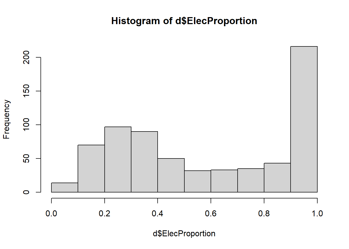
Above, we used the hist function and then simply included a single variable as an argument. This produces a histogram of that variable.
As you can see above, a large proportion of districts have over 90% of its schools with electricity. The bars show how many of the 680 observations in our data fall within the given interval. In this case, each interval is 0.1 in size.
Histograms are very important in predictive analytics, because we need to know the balance between or among the levels of the dependent variable. This concept is highly relevant to the predictive models we will be using later in this course.
4.3.2 Box plot
A box plot also allows us to look at the distribution of a continuous variable. Let’s look at our ElecProportion variable again.
boxplot(d$ElecProportion)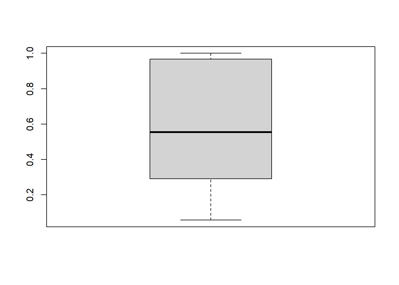
Above, we used the boxplot function and then simply included a single variable as an argument. This produces a box plot of that variable.
A box plot is good at telling us where the majority of our data lies and where any outliers lie relative to the majority. This is well-illustrated by looking at a box plot of SELETOT:
boxplot(d$SELETOT)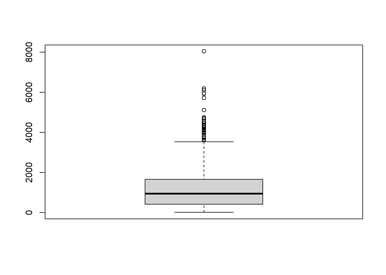
As you can see above, the highest dot in the box plot shows the outlier that we identified earlier in this chapter.
Another visualization that I really like to use box plots for is looking at the distribution of a continuous variable grouped by a discrete (categorical) variable. For example, we can look at ElecProportion across the different states in India:
boxplot(ElecProportion ~ STATNAME,data=d)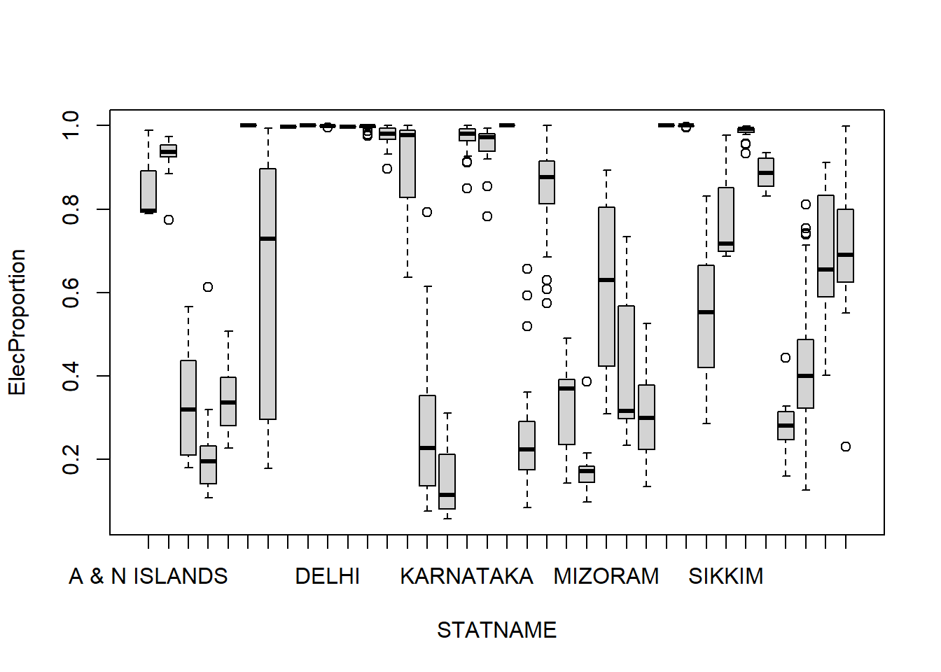
Let’s break down the code from above:
boxplot(...)– This is theboxplotfunction that creates box plots. The information inside the parentheses tells it which data to use and how to organize that data to make a box plot.ElecProportion ~ STATNAME– This is the first argument in theboxplotfunction. It tells the computer that we want to seeElecProportionon the vertical axis (which is usually the axis on which we put our dependent variable, meaning our outcome of interest) and the various groups ofSTATNAMEon the horizontal axis (STATNAMEis the name of the variable that identifies the state in which each district in our data is located).,data=d– This tells the computer where to get the variables that were given in the previous argument. In this case, the variables are found in the datasetd.
Remember that the first variable—ElecProportion in this example—must be a continuous numeric variable. And the second variable—STATNAME in this example—must be a discrete variable.
As you can see above, we created a separate box plot for the variable ElecProportion in each state!15 This can be very useful in telling us that there is extreme variation across the states in terms of the availability of electricity in schools. There is extreme heterogeneity in this variable across states. If the box plot for each state had been identical, then we would know that the situation is fairly similar in each state, meaning that this variable would be more homogeneous.
4.3.3 Other “big data” visualizations (optional)
This entire section is optional (not required) for you to read.
When you are dealing with a huge amount of data, standard visualizations sometimes are not helpful. Depending on the nature and subject matter of the data, sometimes unique contextualized visualizations are necessary. The following article shows examples of these:
- HEAVY.AI Team. Ten Dynamic Examples of Visualizing Big Data. 2020. https://www.heavy.ai/blog/ten-dynamic-examples-of-visualizing-big-data.
In some cases, it is possible to make such visualizations in R. In other cases, additional software or customization is needed.
The following resource also shows examples, with code, of some creative visualizations that are possible in R:
- Chapter 5, “Visualizing big data” in: Bulut, O & Desjardins, C. 2019. Exploring, Visualizing, and Modeling Big Data with R. https://okanbulut.github.io/bigdata/visualizing-big-data.html.
You have now reached the end of this week’s learning materials. Please proceed to the assignment below.
4.4 Assignment
In this assignment, you will use a dataset of your choice to practice some of the preprocessing and visualization techniques that were demonstrated earlier in this chapter.
Please complete the tasks that are below in this assignment. For all of them, please provide any relevant R code in addition to your answer. This can all be done easily in an RMarkdown file, but you can also submit in a different format if you want. Please knit your RMarkdown file and submit the outputted file to D2L.16
What data should you use for this assignment? There are multiple options:
- If you have access to a dataset of your own that would be well-suited to predictive analytics, we encourage you to use it for your assignments in this course. Just do all of the tasks below using that dataset!
- This dataset could come from your own work, your organization/employer, or any other source you would like.
- You are welcome to consult with an instructor if you are not sure how best to proceed. We can meet with you to look at the data that you have and make a recommendation about if or how to use it. It might be necessary to reformat it a little bit before loading it into R.
- For information on how to load Excel format data into R, please refer to Load Excel data into R at https://www.heavy.ai/blog/ten-dynamic-examples-of-visualizing-big-data.
- Those of you who took the course HE-902 should consider using the dataset that you used for your HE-902 final project for the assignments in this course (and maybe even the final project).
- This is a convenient option because you are already familiar with your HE-902 data and you are certain that it can be successfully loaded into R. You can re-use your code from your HE-902 final project to load and prepare your data, if you would like. Then you can apply additional preprocessing techniques in the assignment below.
- You can probably use the same dependent variable as you did in HE-902 for most of HE-930. However, it is also fine to change the dependent variable if you want. Feel free to discuss this with us!
- You can use the
student-por.csvdataset that we explored previously.
4.4.2 Revisit week 2 dashboard assignment
Task 1: At some point during this week, you will receive feedback on your week 2 dashboard assignment. You might be asked to make changes to the dashboard. Please submit your revised dashboard (if required) along with your Week 4 assignment.
4.4.3 Basic dataset characteristics
Now we will turn to our dataset and assignment for this week. To get started, we’ll explore the dataset a little bit.
Task 2: What is the unit of observation in this dataset? In other words, what does each row in the dataset represent?
Task 3: How many observations are in this data?
Task 4: How many variables are in this data?
4.4.4 Research question
Now that you have explored the dataset a little bit more, it is time to decide on a research question that could be useful to study.
Task 5: Write one research question that this dataset could help you answer. Try to write it as a predictive analytics question (one that helps you predict future outcomes), like the examples earlier in this tutorial.
Task 6: In what situation would it be useful to have the answer to this research question?
4.4.5 Pre-processing
In this part of the assignment, you will practice pre-processing your data so that it is ready for use in predictive analysis.
Task 7: Create one new independent or dependent variable from the ones that already exist in the dataset. Explain how this new variable could be useful for answering your research question.
Task 8: Choose one continuous variable that you intend to use as a dependent variable to answer your research question. Discretize this variable and create a new discrete (binary) variable based on it. Use the head command to inspect your work and confirm that the new discretized variable was successfully created.
Task 9: Standardize the entire dataset. Again, use the head command to inspect your work. Was the standardization successful?17
4.4.6 Visualization
Now you will practice generating some visualizations of your data in R.
Task 10: Make a histogram showing the distribution of one or more variables relevant to your research question.
Task 11: Make a box plot showing one or more variables relevant to your research question.
Task 12: Make a box plot that shows the distribution of a continuous variable separately for all levels of a discrete (binary or otherwise categorical) variable. Be sure to choose variables to display that are meaningful to your research question.
Task 13: Brainstorm about and describe (but do not create) a new or unique type of visualization that would be useful to display information about the dataset you are using for this assignment.
Task 14 (optional): This task is not required. It is for extra credit only. Find one visualization that you like from Chapter 5 at https://okanbulut.github.io/bigdata/visualizing-big-data.html. Replicate this visualization for the data you are using for this assignment, choosing variables that would be meaningful to visualize.
4.4.7 Follow-up and submission
You have now reached the end of this week’s assignment. The tasks below will guide you through submission of the assignment and allow us to gather questions and feedback from you.
Task 15: Please write any questions you have for the course instructors (optional). These can relate to this or any other week of the course.
Task 16: Please write any feedback you have about the course and instructional materials from the first few weeks (optional).
Task 17: Please submit your assignment (multiple files are fine) to the D2L assignment drop-box corresponding to this chapter and week of the course. To get to the drop-box, go to the D2L page for this course, click on Assessments -> Assignments. Please e-mail all instructors if you experience any difficulty with this process.
A data frame is the same thing as a dataset. “Data frame” is the technical name for a stored dataset object in R.↩︎
For example, we could have called our dataset
schoolDistricts, in which case we would write the code like this:d <- read.csv("2015_16_Districtwise.csv"). That would be a perfectly reasonable decision. The reason I chose to call the datasetdin this chapter is because it is easier to type quickly and because we are only using a single dataset in the chapter. If we were using many datasets, then I would want to give each one a more descriptive name. This is completely a matter of preference and there is no single correct way to name your dataset(s) when you are using R.↩︎This stands for “d standardized”, but we could have called this anything else we wanted, like
d2orelephants. But usually it makes sense to choose something short and logical.↩︎Not all of the labels appear, but we know that each box plot is for a separate state↩︎
Any knitted format—including Word, HTML, and PDF—is acceptable. It is your choice!↩︎
Note that you could also use the
View(yourdataset)command in the console (not your RMarkdown file) to examine the standardized dataset.↩︎