Capitulo 4 Analisis de Datos
4.1 Reglas de Asociacion
4.1.1 Anotaciones
Notación en market basket analysis
- Datos: Típicamente una matriz binaria D dispersa de tamaño muy grande.
- Item: Cada columna del dataset. Un dato del dataset que puede ser un atributo, una palabra, un documento, un biomarcador, etc.
- Transacción: Cada fila del dataset, representando típicamente un producto.
- Itemset: Una colección de cero o más items.
Minería de Reglas de Asociación
- Confianza: Una medida de la incertidumbre del patrón descubierto.
- Soporte: Una medida de en qué porcentaje el patrón encontrado aparece respecto al tamaño del dataset.
- Frequent itemset: Establecer un umbral respecto al soporte que debe satisfacer el itemset encontrado.
- Strong Association rules: Reglas que satisfacen umbrales de soporte y de confianza.
Extracción de Reglas
El numero de posibles reglas con d atributos es: \(numreglas = 3^d-2^{d+1}+1\)
Soporte: \(Sop(X) = \frac{\mid X\mid}{\mid D\mid}\) con \({\mid X\mid}\) número de filas con X y \({\mid D\mid}\) el número de filas de la tabla.
- El soporte denota la frecuencia de la regla en el dataset, \(P(X\cup Y)\).
- Un alto valor indica que la regla es cierta en gran parte de la base de datos.
- Un bajo valor indica una regla poco frecuente. Podríamos descartar las reglas con bajo soporte.
Confianza: \(Conf(X \rightarrow Y) = \frac{Sop(X \cup Y)}{Sop(X)} = \frac{\mid X \cup Y \mid}{\mid X\mid}\)
- La confianza es un estimador de la \(P(X/Y)\), es decir, el porcentaje del dataset que conteniendo X también contiene a Y.
- Es un indicador de la fiabilidad de la regla.
Lift: \(Lift(X \rightarrow Y) = \frac{Sop(X \cup Y)}{Sop(X)Sop(Y)}\) * X e Y están negativamente correlacionados si el valor es menor que 1. * Es simétrica: \(X \rightarrow Y, Y \rightarrow X\) tienen igual Lift.
Conviction \(Conv(X \rightarrow Y) = \frac{Sop(X)Sop(\overline Y)}{Sop(X \cup \overline Y)}\) * Conv valdrá 1 si los items X e Y no están relacionados.
Leverage - Piatetsky-Shapiro \(Lev(X \rightarrow Y) = Sop(X \cup Y)-Sop(X)Sop(Y)\)
4.1.2 Ejercicio diapositiva
# Este es el ejercicio que habia que realizar a mano. Esta aqui para comprobar el resultado.
library(arules)
## Loading required package: Matrix##
## Attaching package: 'arules'## The following object is masked from 'package:dplyr':
##
## recode## The following objects are masked from 'package:base':
##
## abbreviate, writeds <- matrix(data = c(1,1,1,1,0,0,0,0,
1,0,0,0,1,1,1,0,
0,1,0,0,1,1,0,1,
1,1,1,0,1,1,0,0,
1,1,0,0,0,1,0,1,
1,1,0,1,1,1,0,0,
1,1,0,0,0,1,0,1),
nrow = 7,ncol = 8, byrow = TRUE)
colnames(ds) <- c("Pan", "Leche", "Patatas", "Mostaza", "Cerveza", "Pañales", "Huevos", "Cola")
rownames(ds) <- 1:7
reglas <- apriori(ds, parameter = list(supp = 0.6, conf = 0.80))## Apriori
##
## Parameter specification:
## confidence minval smax arem aval originalSupport maxtime support minlen
## 0.8 0.1 1 none FALSE TRUE 5 0.6 1
## maxlen target ext
## 10 rules FALSE
##
## Algorithmic control:
## filter tree heap memopt load sort verbose
## 0.1 TRUE TRUE FALSE TRUE 2 TRUE
##
## Absolute minimum support count: 4
##
## set item appearances ...[0 item(s)] done [0.00s].
## set transactions ...[8 item(s), 7 transaction(s)] done [0.00s].
## sorting and recoding items ... [3 item(s)] done [0.00s].
## creating transaction tree ... done [0.00s].
## checking subsets of size 1 2 3 done [0.00s].
## writing ... [9 rule(s)] done [0.00s].
## creating S4 object ... done [0.00s].4.1.3 Ejemplo titanic diapositivas
## [1] "data.frame"## Class Sex Age Survived
## 1st :325 Female: 470 Adult:2092 No :1490
## 2nd :285 Male :1731 Child: 109 Yes: 711
## 3rd :706
## Crew:885## Class Sex Age Survived
## 1657 3rd Male Adult Yes
## 1784 Crew Male Adult Yes
## 518 3rd Male Adult No
## 2004 1st Female Adult Yes
## 180 2nd Male Adult Nolibrary(arules)
# el dataset es de tipo Transactions (binary o data.frame)
# las reglas generadas tienen siempre a la derecha 1 item
mis.reglas <- apriori(titanic.raw) ## Apriori
##
## Parameter specification:
## confidence minval smax arem aval originalSupport maxtime support minlen
## 0.8 0.1 1 none FALSE TRUE 5 0.1 1
## maxlen target ext
## 10 rules FALSE
##
## Algorithmic control:
## filter tree heap memopt load sort verbose
## 0.1 TRUE TRUE FALSE TRUE 2 TRUE
##
## Absolute minimum support count: 220
##
## set item appearances ...[0 item(s)] done [0.00s].
## set transactions ...[10 item(s), 2201 transaction(s)] done [0.00s].
## sorting and recoding items ... [9 item(s)] done [0.00s].
## creating transaction tree ... done [0.00s].
## checking subsets of size 1 2 3 4 done [0.00s].
## writing ... [27 rule(s)] done [0.00s].
## creating S4 object ... done [0.00s].## lhs rhs support confidence
## [1] {} => {Age=Adult} 0.9504771 0.9504771
## [2] {Class=2nd} => {Age=Adult} 0.1185825 0.9157895
## [3] {Class=1st} => {Age=Adult} 0.1449341 0.9815385
## [4] {Sex=Female} => {Age=Adult} 0.1930940 0.9042553
## [5] {Class=3rd} => {Age=Adult} 0.2848705 0.8881020
## [6] {Survived=Yes} => {Age=Adult} 0.2971377 0.9198312
## [7] {Class=Crew} => {Sex=Male} 0.3916402 0.9740113
## [8] {Class=Crew} => {Age=Adult} 0.4020900 1.0000000
## [9] {Survived=No} => {Sex=Male} 0.6197183 0.9154362
## [10] {Survived=No} => {Age=Adult} 0.6533394 0.9651007
## [11] {Sex=Male} => {Age=Adult} 0.7573830 0.9630272
## [12] {Sex=Female,Survived=Yes} => {Age=Adult} 0.1435711 0.9186047
## [13] {Class=3rd,Sex=Male} => {Survived=No} 0.1917310 0.8274510
## [14] {Class=3rd,Survived=No} => {Age=Adult} 0.2162653 0.9015152
## [15] {Class=3rd,Sex=Male} => {Age=Adult} 0.2099046 0.9058824
## [16] {Sex=Male,Survived=Yes} => {Age=Adult} 0.1535666 0.9209809
## [17] {Class=Crew,Survived=No} => {Sex=Male} 0.3044071 0.9955423
## [18] {Class=Crew,Survived=No} => {Age=Adult} 0.3057701 1.0000000
## [19] {Class=Crew,Sex=Male} => {Age=Adult} 0.3916402 1.0000000
## [20] {Class=Crew,Age=Adult} => {Sex=Male} 0.3916402 0.9740113
## [21] {Sex=Male,Survived=No} => {Age=Adult} 0.6038164 0.9743402
## [22] {Age=Adult,Survived=No} => {Sex=Male} 0.6038164 0.9242003
## [23] {Class=3rd,Sex=Male,Survived=No} => {Age=Adult} 0.1758292 0.9170616
## [24] {Class=3rd,Age=Adult,Survived=No} => {Sex=Male} 0.1758292 0.8130252
## [25] {Class=3rd,Sex=Male,Age=Adult} => {Survived=No} 0.1758292 0.8376623
## [26] {Class=Crew,Sex=Male,Survived=No} => {Age=Adult} 0.3044071 1.0000000
## [27] {Class=Crew,Age=Adult,Survived=No} => {Sex=Male} 0.3044071 0.9955423
## lift count
## [1] 1.0000000 2092
## [2] 0.9635051 261
## [3] 1.0326798 319
## [4] 0.9513700 425
## [5] 0.9343750 627
## [6] 0.9677574 654
## [7] 1.2384742 862
## [8] 1.0521033 885
## [9] 1.1639949 1364
## [10] 1.0153856 1438
## [11] 1.0132040 1667
## [12] 0.9664669 316
## [13] 1.2222950 422
## [14] 0.9484870 476
## [15] 0.9530818 462
## [16] 0.9689670 338
## [17] 1.2658514 670
## [18] 1.0521033 673
## [19] 1.0521033 862
## [20] 1.2384742 862
## [21] 1.0251065 1329
## [22] 1.1751385 1329
## [23] 0.9648435 387
## [24] 1.0337773 387
## [25] 1.2373791 387
## [26] 1.0521033 670
## [27] 1.2658514 670## Apriori
##
## Parameter specification:
## confidence minval smax arem aval originalSupport maxtime support minlen
## 1 0.1 1 none FALSE TRUE 5 0.005 1
## maxlen target ext
## 10 rules FALSE
##
## Algorithmic control:
## filter tree heap memopt load sort verbose
## 0.1 TRUE TRUE FALSE TRUE 2 TRUE
##
## Absolute minimum support count: 11
##
## set item appearances ...[0 item(s)] done [0.00s].
## set transactions ...[10 item(s), 2201 transaction(s)] done [0.00s].
## sorting and recoding items ... [10 item(s)] done [0.00s].
## creating transaction tree ... done [0.00s].
## checking subsets of size 1 2 3 4 done [0.00s].
## writing ... [18 rule(s)] done [0.00s].
## creating S4 object ... done [0.00s].## lhs rhs support confidence lift
## [1] {Class=Crew} => {Age=Adult} 0.40208996 1 1.052103
## [2] {Class=2nd,Age=Child} => {Survived=Yes} 0.01090413 1 3.095640
## [3] {Age=Child,Survived=No} => {Class=3rd} 0.02362562 1 3.117564
## [4] {Class=2nd,Survived=No} => {Age=Adult} 0.07587460 1 1.052103
## [5] {Class=1st,Survived=No} => {Age=Adult} 0.05542935 1 1.052103
## [6] {Class=Crew,Sex=Female} => {Age=Adult} 0.01044980 1 1.052103
## count
## [1] 885
## [2] 24
## [3] 52
## [4] 167
## [5] 122
## [6] 23# Solo extrae reglas con un atributo a la derecha
# con un valor concreto
mis.reglas3 <- apriori(titanic.raw,parameter = list(supp=0.005, conf=1), appearance = list(rhs=c("Survived=Yes"))) ## Apriori
##
## Parameter specification:
## confidence minval smax arem aval originalSupport maxtime support minlen
## 1 0.1 1 none FALSE TRUE 5 0.005 1
## maxlen target ext
## 10 rules FALSE
##
## Algorithmic control:
## filter tree heap memopt load sort verbose
## 0.1 TRUE TRUE FALSE TRUE 2 TRUE
##
## Absolute minimum support count: 11
##
## set item appearances ...[1 item(s)] done [0.00s].
## set transactions ...[10 item(s), 2201 transaction(s)] done [0.00s].
## sorting and recoding items ... [10 item(s)] done [0.00s].
## creating transaction tree ... done [0.00s].
## checking subsets of size 1 2 3 4 done [0.00s].
## writing ... [2 rule(s)] done [0.00s].
## creating S4 object ... done [0.00s].## lhs rhs support confidence
## [1] {Class=2nd,Age=Child} => {Survived=Yes} 0.010904134 1
## [2] {Class=2nd,Sex=Female,Age=Child} => {Survived=Yes} 0.005906406 1
## lift count
## [1] 3.09564 24
## [2] 3.09564 13# MAS POSIBILIDADES
rules <- apriori(titanic.raw, control = list(verbose=F), parameter = list(minlen=3, supp=0.002, conf=0.2), appearance = list( rhs=c("Survived=Yes"), lhs=c("Class=1st", "Class=2nd", "Class=3rd", "Age=Child", "Age=Adult")))
rules.sorted <- sort(rules, by="confidence")
inspect(rules.sorted)## lhs rhs support confidence lift
## [1] {Class=2nd,Age=Child} => {Survived=Yes} 0.010904134 1.0000000 3.0956399
## [2] {Class=1st,Age=Child} => {Survived=Yes} 0.002726034 1.0000000 3.0956399
## [3] {Class=1st,Age=Adult} => {Survived=Yes} 0.089504771 0.6175549 1.9117275
## [4] {Class=2nd,Age=Adult} => {Survived=Yes} 0.042707860 0.3601533 1.1149048
## [5] {Class=3rd,Age=Child} => {Survived=Yes} 0.012267151 0.3417722 1.0580035
## [6] {Class=3rd,Age=Adult} => {Survived=Yes} 0.068605179 0.2408293 0.7455209
## count
## [1] 24
## [2] 6
## [3] 197
## [4] 94
## [5] 27
## [6] 1514.1.4 Ejercicio Soporte y Confianza
Trabajando con el paquete arules
- Objetivo y ejemplo de ejecución
## Apriori
##
## Parameter specification:
##  confidence minval smax arem  aval originalSupport maxtime support minlen
##           1    0.1    1 none FALSE            TRUE       5     0.1      1
##  maxlen target   ext
##      10  rules FALSE
##
## Algorithmic control:
##  filter tree heap memopt load sort verbose
##     0.1 TRUE TRUE  FALSE TRUE    2    TRUE
##
## Absolute minimum support count: 4884
##
## set item appearances ...[0 item(s)] done [0.00s].
## set transactions ...[115 item(s), 48842 transaction(s)] done [0.03s].
## sorting and recoding items ... [31 item(s)] done [0.01s].
## creating transaction tree ... done [0.02s].
## checking subsets of size 1 2 3 4 5 6 7 8 9 done [0.07s].
## writing ... [72 rule(s)] done [0.00s].
## creating S4 object ... done [0.00s].## lhs rhs support confidence lift count
## [1] {relationship=Husband,
## hours-per-week=Over-time,
## native-country=United-States} => {sex=Male} 0.1366447 1 1.495926 6674dado el dataset Adult del que se han generado reglas de asociación,
a reg1 por error le hemos borrado el soporte y la confianza
##    support confidence     lift count
## 10       0          0 1.495926  6674
Escribir una función computer_suppport_confidence que dado un dataset y una regla de asociación obtenida a partir del dataset con el comando apriori, obtenga:
soporte(\(X \cup Y\)) (soporte de la unión de X e Y)
confianza(X -> Y)
Y estos valores calculados visto en en clase se almacenen en la regla.
La función tendría el siguiente formato:
computer_suppport_confidence <- function(Dataset, Rule1){
....
return(list( my.soporte=....., my.confidence=.....   ))

}
computer_suppport_confidence <- function(Dataset, Rule1){
vector_items <- unlist(as(items(Rule1), "list"))
vector_izq <- unlist(as(lhs(Rule1), "list"))
filtrado_transacciones_soporte <- subset(x = Dataset,
subset = items %ain% vector_items)
soporteXUY <- length(filtrado_transacciones_soporte)/length(Dataset)
filtrado_transacciones_confidence <- subset(x = Dataset,
subset = items %ain% vector_izq)
soporteX <- length(filtrado_transacciones_confidence)/length(Dataset)
confidence <- soporteXUY/soporteX
return(list( my.soporte=soporteXUY,
my.confidence=confidence))
}4.1.5 Ejercicio aleatorio de reglas de asociacion
library(arules)
data <- read.transactions("Groceries65")

reglas <- apriori(data, parameter = list(supp = 0.001, conf = 0.6))
## Apriori
##
## Parameter specification:
## confidence minval smax arem aval originalSupport maxtime support minlen
## 0.6 0.1 1 none FALSE TRUE 5 0.001 1
## maxlen target ext
## 10 rules FALSE
##
## Algorithmic control:
## filter tree heap memopt load sort verbose
## 0.1 TRUE TRUE FALSE TRUE 2 TRUE
##
## Absolute minimum support count: 6
##
## set item appearances ...[0 item(s)] done [0.00s].
## set transactions ...[169 item(s), 6393 transaction(s)] done [0.00s].
## sorting and recoding items ... [155 item(s)] done [0.00s].
## creating transaction tree ... done [0.00s].
## checking subsets of size 1 2 3 4 5 6 done [0.01s].
## writing ... [3756 rule(s)] done [0.00s].
## creating S4 object ... done [0.00s].## lhs rhs support confidence
## [1] {beef,pickled vegetables} => {other vegetables} 0.001720632 0.6470588
## lift count
## [1] 3.430056 11# Ordenamos las reglas por confianza
reglas <- sort(reglas, by = "confidence")
inspect(reglas[1:20])## lhs rhs support confidence lift count
## [1] {cereals,
## tropical fruit} => {whole milk} 0.001251369 1 3.917279 8
## [2] {house keeping products,
## napkins} => {whole milk} 0.001094948 1 3.917279 7
## [3] {rice,
## sugar} => {whole milk} 0.001407790 1 3.917279 9
## [4] {bottled water,
## rice} => {whole milk} 0.001094948 1 3.917279 7
## [5] {canned fish,
## hygiene articles} => {whole milk} 0.001407790 1 3.917279 9
## [6] {cat food,
## frozen vegetables} => {other vegetables} 0.001251369 1 5.300995 8
## [7] {liquor,
## red/blush wine,
## soda} => {bottled beer} 0.001251369 1 11.949533 8
## [8] {cereals,
## curd,
## yogurt} => {whole milk} 0.001094948 1 3.917279 7
## [9] {cereals,
## curd,
## whole milk} => {yogurt} 0.001094948 1 7.231900 7
## [10] {rice,
## root vegetables,
## yogurt} => {whole milk} 0.001407790 1 3.917279 9
## [11] {beef,
## mayonnaise,
## other vegetables} => {root vegetables} 0.001094948 1 9.265217 7
## [12] {dishes,
## root vegetables,
## whole milk} => {other vegetables} 0.001407790 1 5.300995 9
## [13] {brown bread,
## herbs,
## whole milk} => {other vegetables} 0.001094948 1 5.300995 7
## [14] {citrus fruit,
## herbs,
## tropical fruit} => {other vegetables} 0.001094948 1 5.300995 7
## [15] {beverages,
## tropical fruit,
## whipped/sour cream} => {other vegetables} 0.001094948 1 5.300995 7
## [16] {fruit/vegetable juice,
## root vegetables,
## semi-finished bread} => {whole milk} 0.001094948 1 3.917279 7
## [17] {curd,
## flour,
## sugar} => {whole milk} 0.001251369 1 3.917279 8
## [18] {flour,
## margarine,
## root vegetables} => {whole milk} 0.001094948 1 3.917279 7
## [19] {flour,
## root vegetables,
## whipped/sour cream} => {whole milk} 0.001877053 1 3.917279 12
## [20] {ice cream,
## newspapers,
## root vegetables} => {other vegetables} 0.001094948 1 5.300995 7# Subset con los elementos cuya confianza sea superior
rules2 <- subset(reglas, subset = (confidence > 0.7))
# Ordenamos las reglas por lift e inspeccionamos las primeras reglas, aunque solo hay que elegir la primera regla,
# consulto el resto para poder ver que el lift es superior en el resto
rules2 <- sort(rules2, by = "lift")
inspect(rules2[1:5])## lhs rhs support confidence lift count
## [1] {bottled beer,
## liquor,
## soda} => {red/blush wine} 0.001251369 0.8000000 41.92131 8
## [2] {curd,
## other vegetables,
## whipped/sour cream,
## whole milk,
## yogurt} => {cream cheese} 0.001407790 0.8181818 22.16371 9
## [3] {curd,
## root vegetables,
## whipped/sour cream,
## yogurt} => {cream cheese} 0.001094948 0.7777778 21.06921 7
## [4] {sugar,
## whipped/sour cream,
## whole milk,
## yogurt} => {curd} 0.001251369 0.8888889 17.70301 8
## [5] {ham,
## specialty bar} => {white bread} 0.001094948 0.7777778 17.02854 74.1.6 Analisis del rmd de Daniel Redondo
En el siguiente enlance encontramos un rmd relativo a reglas de asociacion elaborado por Daniel Redondo:
https://danielredondo.com/posts/20200405_reglas_asociacion/
A lo largo del rmd podemos ver las mismas tecnicas estudiadas en clase, y podría destacar unicamente la siguiente funcion no vista:
interesMeasure
Esta funcion proporciona:
Si solo se usa una medida, la función devuelve un vector numérico que contiene los valores de la medida de interés para cada asociación en el conjunto de asociaciones x.
Si se especifican más de una medida, el resultado es un data.frame que contiene las diferentes medidas para cada asociación como columnas.
NA se devuelve para reglas / conjuntos de elementos para los que no se define una determinada medida.
Esta funcion tiene un parametro llamado measure, el cual indica las medidas de interes que queremos aplicar. Existen un gran numero de posbiles medidads implementadas, sin embargo, en el rmd estudiado hace uso de measure = c(“gini”, “chiSquared”).
gini mide la entropía cuadrática de una regla, y chiSquared sirve para probar la independencia entre las lhs y rhs de la regla. Los valores de chi-cuadrado más altos indican que lhs y rhs no son independientes
4.1.7 Ejercicio Iris
Analizando el dataset Iris
- Cargar en R el dataset Iris.
- Utilizar las funciones que se han visto para analizar el dataset, ver número de transacciones, items del dataset, información estadística del dataset. NOTA: dataset debe ser preprocesado. Discretizar de tres formas: transformando el tipo de las variables (convirtiendo a factor), discretizando los datos (convirtiendo en categóricos), y usando el comando discretize. Guardar los resultados en tres datasets. Consulta la ayuda de arules para discretize.
# Cargamos iris en los tres datasets, para luego modificar cada uno.
ds1 <- ds2 <- ds3 <- iris

## Usando factores
factor_sepal_length = cut(iris$Sepal.Length, breaks = 3,
                          labels = c("S_short", "S_medium", "S_long"),
                          include.lowest = TRUE)

factor_sepal_width = cut(iris$Sepal.Width, breaks = 3,
                         labels = c("S_thin", "S_medium", "S_wide"),
                         include.lowest = TRUE)

factor_petal_length = cut(iris$Petal.Length, breaks = 3,
                          labels = c("P_short", "P_medium", "P_long"),
                          include.lowest = TRUE)

factor_petal_width = cut(iris$Petal.Width, breaks = 3,
                         labels = c("P_thin", "P_medium", "P_wide"),
                         include.lowest = TRUE)

# Cargamos los nuevos datos en el dataset, siendo todos de tipo factor.
ds1$Sepal.Length <- factor_sepal_length
ds1$Sepal.Width <- factor_sepal_width
ds1$Petal.Length <- factor_petal_length
ds1$Petal.Width <- factor_petal_width

paged_table(ds1)
# Conversion a transactions
ds1 <- as(ds1, "transactions")
## Conversion a variables categoricas
i <- (max(iris$Sepal.Length)-min(iris$Sepal.Length))/3
base <- min(iris$Sepal.Length)
c1 <- c(base, base+i, base+i*2)
ds2$Sepal.Length[iris$Sepal.Length < c1[2]] <- "S_short"
ds2$Sepal.Length[iris$Sepal.Length >= c1[2] & iris$Sepal.Length < c1[3]] <- "S_medium"
ds2$Sepal.Length[iris$Sepal.Length >= c1[3]] <- "S_long"
ds2$Sepal.Length <- factor(ds2$Sepal.Length)
i <- (max(iris$Sepal.Width)-min(iris$Sepal.Width))/3
base <- min(iris$Sepal.Width)
c2 <- c(base, base+i, base+i*2)
ds2$Sepal.Width[iris$Sepal.Width < c2[2]] <- "S_thin"
ds2$Sepal.Width[iris$Sepal.Width >= c2[2] & iris$Sepal.Width < c2[3]] <- "S_medium"
ds2$Sepal.Width[iris$Sepal.Width >= c2[3]] <- "S_wide"
ds2$Sepal.Width <- factor(ds2$Sepal.Width)
i <- (max(iris$Petal.Length)-min(iris$Petal.Length))/3
base <- min(iris$Petal.Length)
c3 <- c(base, base+i, base+i*2)
ds2$Petal.Length[iris$Petal.Length < c3[2]] <- "P_short"
ds2$Petal.Length[iris$Petal.Length >= c3[2] & iris$Petal.Length < c3[3]] <- "P_medium"
ds2$Petal.Length[iris$Petal.Length >= c3[3]] <- "P_long"
ds2$Petal.Length <- factor(ds2$Petal.Length)
i <- (max(iris$Petal.Width)-min(iris$Petal.Width))/3
base <- min(iris$Petal.Width)
c4 <- c(base, base+i, base+i*2)
ds2$Petal.Width[iris$Petal.Width < c4[2]] <- "P_thin"
ds2$Petal.Width[iris$Petal.Width >= c4[2] & iris$Petal.Width < c4[3]] <- "P_medium"
ds2$Petal.Width[iris$Petal.Width >= c4[3]] <- "P_wide"
ds2$Petal.Width <- factor(ds2$Petal.Width)
paged_table(ds2)# Conversion a transactions
ds2 <- as(ds2, "transactions")
## Usando el metodo discretize
# Este será el dataset que usaremos a lo largo del ejercicio
ds3$Sepal.Length <- discretize(iris$Sepal.Length,
labels = c("S_short", "S_medium", "S_long"),
method = "frequency", breaks = 3, include.lowest = TRUE)
ds3$Sepal.Width <- discretize(iris$Sepal.Width,
labels = c("S_thin", "S_medium", "S_wide"),
method = "frequency", breaks = 3, include.lowest = TRUE)
ds3$Petal.Length <- discretize(iris$Petal.Length,
labels = c("P_short", "P_medium", "P_long"),
method = "frequency", breaks = 3, include.lowest = TRUE)
ds3$Petal.Width <- discretize(iris$Petal.Width,
labels = c("P_thin", "P_medium", "P_wide"),
method = "frequency", breaks = 3, include.lowest = TRUE)
paged_table(ds3)# Conversion a transactions
ds3 <- as(ds3, "transactions")
# Numero de transacciones (Filas) e items (Columnas)
transacciones <- nrow(ds3)
transacciones## [1] 150## [1] 15## transactions as itemMatrix in sparse format with
## 150 rows (elements/itemsets/transactions) and
## 15 columns (items) and a density of 0.3333333
##
## most frequent items:
## Sepal.Width=S_wide Sepal.Length=S_medium Petal.Width=P_wide
## 56 53 52
## Sepal.Length=S_long Petal.Length=P_long (Other)
## 51 51 487
##
## element (itemset/transaction) length distribution:
## sizes
## 5
## 150
##
## Min. 1st Qu. Median Mean 3rd Qu. Max.
## 5 5 5 5 5 5
##
## includes extended item information - examples:
## labels variables levels
## 1 Sepal.Length=S_short Sepal.Length S_short
## 2 Sepal.Length=S_medium Sepal.Length S_medium
## 3 Sepal.Length=S_long Sepal.Length S_long
##
## includes extended transaction information - examples:
## transactionID
## 1 1
## 2 2
## 3 3- Utilizar algoritmo apriori para obtener las reglas de asociación con confianza 0.5 y soporte 0.01. LLamar estas reglas r1.
## Apriori
##
## Parameter specification:
##  confidence minval smax arem  aval originalSupport maxtime support minlen
##         0.5    0.1    1 none FALSE            TRUE       5    0.01      1
##  maxlen target   ext
##      10  rules FALSE
##
## Algorithmic control:
##  filter tree heap memopt load sort verbose
##     0.1 TRUE TRUE  FALSE TRUE    2    TRUE
##
## Absolute minimum support count: 1
##
## set item appearances ...[0 item(s)] done [0.00s].
## set transactions ...[15 item(s), 150 transaction(s)] done [0.00s].
## sorting and recoding items ... [15 item(s)] done [0.00s].
## creating transaction tree ... done [0.00s].
## checking subsets of size 1 2 3 4 5 done [0.00s].
## writing ... [532 rule(s)] done [0.00s].
## creating S4 object ... done [0.00s].- Encontrar reglas redundantes en r1 de dos formas distintas. Eliminarlas. Guardar en una variable las redundantes. Buscar en el paquete arules una función que te calcula las reglas redundantes.
Apunte: Una regla será redundante si existen reglas mas generales con la misma o mayor confianza, es decir, una regla más especifica es redundante si es igual o incluso menos predictiva que una regla más general. Una regla es mas general si tiene la misma RHS pero uno o mas itemas de la LHS son eliminados. Una regla \(X \Rightarrow Y\) es redundante si:
# Guardando las reglas redundantes
# Hacemos uso de la funcion del paquete arules is.redundant
idxRed <- which(is.redundant(r1))
vRed <- r1[idxRed]
vRed
## set of 336 rules# Guardando en r1 las reglas sin redundancia
idxNoRed <- which(!is.redundant(r1))
r1 <- r1[idxNoRed]
r1## set of 196 rules- Generar 3 conjuntos de reglas que cumplan que ciertos valores estén a la izquierda y/o derecha. Llamarlas r2,r3,r4.
# Valores en la izquierda
r2 <- apriori(ds3,
              parameter = list(supp = 0.01, conf = 0.50),
              appearance = list(default="rhs",lhs="Sepal.Length=S_short"))
## Apriori
##
## Parameter specification:
## confidence minval smax arem aval originalSupport maxtime support minlen
## 0.5 0.1 1 none FALSE TRUE 5 0.01 1
## maxlen target ext
## 10 rules FALSE
##
## Algorithmic control:
## filter tree heap memopt load sort verbose
## 0.1 TRUE TRUE FALSE TRUE 2 TRUE
##
## Absolute minimum support count: 1
##
## set item appearances ...[1 item(s)] done [0.00s].
## set transactions ...[15 item(s), 150 transaction(s)] done [0.00s].
## sorting and recoding items ... [15 item(s)] done [0.00s].
## creating transaction tree ... done [0.00s].
## checking subsets of size 1 2 done [0.00s].
## writing ... [4 rule(s)] done [0.00s].
## creating S4 object ... done [0.00s].# Valores en la derecha
r3 <- apriori(ds3,
parameter = list(supp = 0.01, conf = 0.50),
appearance = list(rhs="Species=setosa",default = "lhs"))## Apriori
##
## Parameter specification:
## confidence minval smax arem aval originalSupport maxtime support minlen
## 0.5 0.1 1 none FALSE TRUE 5 0.01 1
## maxlen target ext
## 10 rules FALSE
##
## Algorithmic control:
## filter tree heap memopt load sort verbose
## 0.1 TRUE TRUE FALSE TRUE 2 TRUE
##
## Absolute minimum support count: 1
##
## set item appearances ...[1 item(s)] done [0.00s].
## set transactions ...[15 item(s), 150 transaction(s)] done [0.00s].
## sorting and recoding items ... [15 item(s)] done [0.00s].
## creating transaction tree ... done [0.00s].
## checking subsets of size 1 2 3 4 5 done [0.00s].
## writing ... [29 rule(s)] done [0.00s].
## creating S4 object ... done [0.00s].# Valores en ambos lados
r4 <- apriori(ds3,
parameter = list(supp = 0.01, conf = 0.50),
appearance = list(rhs="Species=setosa", lhs="Petal.Width=P_thin"))## Apriori
##
## Parameter specification:
## confidence minval smax arem aval originalSupport maxtime support minlen
## 0.5 0.1 1 none FALSE TRUE 5 0.01 1
## maxlen target ext
## 10 rules FALSE
##
## Algorithmic control:
## filter tree heap memopt load sort verbose
## 0.1 TRUE TRUE FALSE TRUE 2 TRUE
##
## Absolute minimum support count: 1
##
## set item appearances ...[2 item(s)] done [0.00s].
## set transactions ...[2 item(s), 150 transaction(s)] done [0.00s].
## sorting and recoding items ... [2 item(s)] done [0.00s].
## creating transaction tree ... done [0.00s].
## checking subsets of size 1 2 done [0.00s].
## writing ... [1 rule(s)] done [0.00s].
## creating S4 object ... done [0.00s].- Unir r2 y r3 y buscar reglas duplicadas y reglas redundantes.
# Haremos uso del operador c()
unionR2R3 <- c(r2,r3)

# Eliminar duplicados
unionR2R3 <- arules::unique(unionR2R3)
unionR2R3
## set of 32 rules# Eliminar reglas redundantes
idx <- which(is.redundant(unionR2R3))
unionR2R3 <- unionR2R3[-idx]
inspect(unionR2R3)## lhs rhs support confidence lift count
## [1] {Sepal.Length=S_short} => {Petal.Length=P_short} 0.26666667 0.8695652 2.608696 40
## [2] {Sepal.Length=S_short} => {Petal.Width=P_thin} 0.26666667 0.8695652 2.608696 40
## [3] {Sepal.Length=S_short} => {Species=setosa} 0.26666667 0.8695652 2.608696 40
## [4] {Sepal.Length=S_short} => {Sepal.Width=S_wide} 0.18666667 0.6086957 1.630435 28
## [5] {Petal.Length=P_short} => {Species=setosa} 0.33333333 1.0000000 3.000000 50
## [6] {Petal.Width=P_thin} => {Species=setosa} 0.33333333 1.0000000 3.000000 50
## [7] {Sepal.Width=S_wide} => {Species=setosa} 0.25333333 0.6785714 2.035714 38
## [8] {Sepal.Length=S_short,
## Sepal.Width=S_medium} => {Species=setosa} 0.07333333 1.0000000 3.000000 11
## [9] {Sepal.Length=S_short,
## Sepal.Width=S_wide} => {Species=setosa} 0.18666667 1.0000000 3.000000 28
## [10] {Sepal.Length=S_medium,
## Sepal.Width=S_wide} => {Species=setosa} 0.06666667 0.7692308 2.307692 10- Hacer la intersección de r2 y r3.
##     lhs                       rhs              support   confidence lift
## [1] {Sepal.Length=S_short} => {Species=setosa} 0.2666667 0.8695652  2.608696
##     count
## [1] 40- Usa subset para inspeccionar las reglas con distintas condiciones.
# Ejemplos del uso de subset
sub <- subset(r1, subset = lift > 3)
# inspect(sub)

# Uso de %in% para seleccionar todas las reglas que contengan species=setosa en el consecuente.
sub1 <- subset(r1, subset = rhs %in% "Species=setosa")
inspect(sub1)
## lhs rhs support confidence lift count
## [1] {Sepal.Length=S_short} => {Species=setosa} 0.26666667 0.8695652 2.608696 40
## [2] {Petal.Length=P_short} => {Species=setosa} 0.33333333 1.0000000 3.000000 50
## [3] {Petal.Width=P_thin} => {Species=setosa} 0.33333333 1.0000000 3.000000 50
## [4] {Sepal.Width=S_wide} => {Species=setosa} 0.25333333 0.6785714 2.035714 38
## [5] {Sepal.Length=S_short,
## Sepal.Width=S_medium} => {Species=setosa} 0.07333333 1.0000000 3.000000 11
## [6] {Sepal.Length=S_short,
## Sepal.Width=S_wide} => {Species=setosa} 0.18666667 1.0000000 3.000000 28
## [7] {Sepal.Length=S_medium,
## Sepal.Width=S_wide} => {Species=setosa} 0.06666667 0.7692308 2.307692 10# Uso de %pin%, selccion parcial, para todos los items que contengan petal.length en rhs
sub2 <- subset(r1, subset = rhs %pin% "Petal.Length=") # 41 resultados
# inspect(sub2)
# Uso de %ain% para seleccionar solo las reglas que tengan items con "Sepal.Length=S_short","Sepal.Width=S_medium" en lhs
sub3 <- subset(r1, subset=lhs%ain%c("Sepal.Length=S_short","Sepal.Width=S_medium"))
inspect(sub3)## lhs rhs support confidence lift count
## [1] {Sepal.Length=S_short,
## Sepal.Width=S_medium} => {Petal.Length=P_short} 0.07333333 1 3 11
## [2] {Sepal.Length=S_short,
## Sepal.Width=S_medium} => {Petal.Width=P_thin} 0.07333333 1 3 11
## [3] {Sepal.Length=S_short,
## Sepal.Width=S_medium} => {Species=setosa} 0.07333333 1 3 11# Uso de %oin% para seleccionar las reglas que tengan alguno o todos los items en lhs.
sub4 <- subset(r1, subset=lhs%oin%c("Sepal.Length=S_short","Sepal.Width=S_medium"))
inspect(sub4)## lhs rhs support confidence lift count
## [1] {Sepal.Length=S_short} => {Petal.Length=P_short} 0.26666667 0.8695652 2.608696 40
## [2] {Sepal.Length=S_short} => {Petal.Width=P_thin} 0.26666667 0.8695652 2.608696 40
## [3] {Sepal.Length=S_short} => {Species=setosa} 0.26666667 0.8695652 2.608696 40
## [4] {Sepal.Length=S_short} => {Sepal.Width=S_wide} 0.18666667 0.6086957 1.630435 28
## [5] {Sepal.Length=S_short,
## Sepal.Width=S_medium} => {Petal.Length=P_short} 0.07333333 1.0000000 3.000000 11
## [6] {Sepal.Length=S_short,
## Sepal.Width=S_medium} => {Petal.Width=P_thin} 0.07333333 1.0000000 3.000000 11
## [7] {Sepal.Length=S_short,
## Sepal.Width=S_medium} => {Species=setosa} 0.07333333 1.0000000 3.000000 11- Usa summary, sort.
## set of 196 rules
##
## rule length distribution (lhs + rhs):sizes
##   2   3   4
##  51 109  36
##
##    Min. 1st Qu.  Median    Mean 3rd Qu.    Max.
##   2.000   2.000   3.000   2.923   3.000   4.000
##
## summary of quality measures:
##     support          confidence          lift           count
##  Min.   :0.01333   Min.   :0.5000   Min.   :1.339   Min.   : 2.00
##  1st Qu.:0.04000   1st Qu.:0.7025   1st Qu.:2.109   1st Qu.: 6.00
##  Median :0.11333   Median :0.9208   Median :2.713   Median :17.00
##  Mean   :0.13480   Mean   :0.8470   Mean   :2.542   Mean   :20.22
##  3rd Qu.:0.24000   3rd Qu.:1.0000   3rd Qu.:2.951   3rd Qu.:36.00
##  Max.   :0.33333   Max.   :1.0000   Max.   :3.261   Max.   :50.00
##
## mining info:
##  data ntransactions support confidence
##   ds3           150    0.01        0.5
# Ordenado por nivel confianza
sortedR1byConfidence <- sort(r1, by="confidence")
inspect(head(sortedR1byConfidence))## lhs rhs support confidence lift
## [1] {Petal.Length=P_short} => {Petal.Width=P_thin} 0.3333333 1 3
## [2] {Petal.Width=P_thin} => {Petal.Length=P_short} 0.3333333 1 3
## [3] {Petal.Length=P_short} => {Species=setosa} 0.3333333 1 3
## [4] {Species=setosa} => {Petal.Length=P_short} 0.3333333 1 3
## [5] {Petal.Width=P_thin} => {Species=setosa} 0.3333333 1 3
## [6] {Species=setosa} => {Petal.Width=P_thin} 0.3333333 1 3
## count
## [1] 50
## [2] 50
## [3] 50
## [4] 50
## [5] 50
## [6] 50# Ordenado por nivel soporte
# Reglas con soporte alto indican frecuencia de apariencia en el dataset.
sortedR1bySupport <- sort(r1, by="support")
inspect(head(sortedR1bySupport))## lhs rhs support confidence lift
## [1] {Petal.Length=P_short} => {Petal.Width=P_thin} 0.3333333 1 3
## [2] {Petal.Width=P_thin} => {Petal.Length=P_short} 0.3333333 1 3
## [3] {Petal.Length=P_short} => {Species=setosa} 0.3333333 1 3
## [4] {Species=setosa} => {Petal.Length=P_short} 0.3333333 1 3
## [5] {Petal.Width=P_thin} => {Species=setosa} 0.3333333 1 3
## [6] {Species=setosa} => {Petal.Width=P_thin} 0.3333333 1 3
## count
## [1] 50
## [2] 50
## [3] 50
## [4] 50
## [5] 50
## [6] 50Explicar y usar los comandos de paquete arules siguientes: dissimilarity, image, is.redundant, is.significant, itemFrequency.
dissimilarity: Debemos entender en que consiste el cálculo de disimilitud. Esto se corresponde con el cálculo de falta de semejanza entre dos objetos principalmente. Este cálculo es facilitado por la funcion dissimilarity y el método S4* para computar y devolver las distancias en matrices de datos binarios, transacciones o asociaciones que pueden ser utilizadas para agrupamiento o clustering.
S4*: El sistema S4 de R es un sistema para la programación orientada a objetos. Este sistema es de utilidad para reconocer objetos S4 y para aprender características o factores para saber como explorar, manipular y usar la ayuda del sistema cuando encontramos clases y métodos S4.
##           1         2         3
## 2 0.6666667
## 3 0.6666667 0.6666667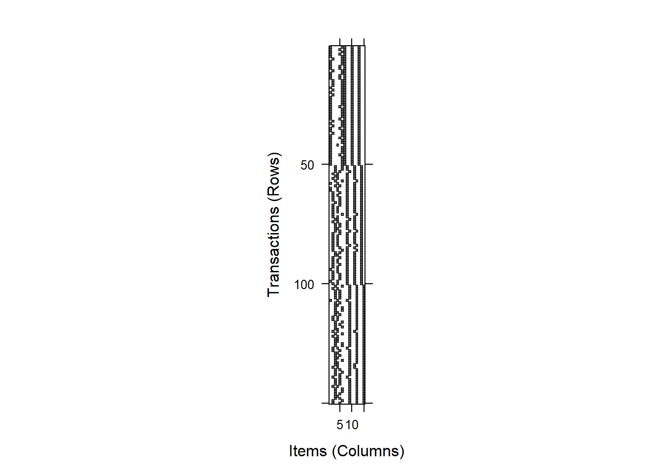
## 4 0.6666667 0.6666667 0.6666667- image: Se trata de una funcion capaz de generar gráficos de nivel para inspeccionar visualmente matrices de incidencia binarias, es decir, objetos basados en itemMatrix (por ejemplo, transacciones, tidLists, items en itemsets o rhs/lhs en reglas). Estos gráficos se pueden usar para identificar problemas en un conjunto de datos (por ejemplo, registrar problemas con algunas transacciones que contienen todos los artículos).
is.redundant: En el ejercicio 4 se realiza una explicacion de lo que significa ser una regla redundante. Este metodo del paquete arules nos permite extraer las reglas que son redundantes dentro de un conjunto de reglas.
is.significant: Sirve para encontrar reglas donde LHS y RHS dependen el uno del otro. Este método utiliza la prueba exacta de Fisher y corrige las comparaciones múltiples.
##   [1]  TRUE  TRUE  TRUE  TRUE  TRUE  TRUE FALSE FALSE  TRUE  TRUE  TRUE  TRUE
##  [13]  TRUE  TRUE FALSE  TRUE  TRUE  TRUE  TRUE  TRUE  TRUE  TRUE  TRUE  TRUE
##  [25]  TRUE  TRUE  TRUE  TRUE  TRUE  TRUE  TRUE  TRUE  TRUE  TRUE  TRUE  TRUE
##  [37]  TRUE  TRUE  TRUE  TRUE  TRUE  TRUE  TRUE  TRUE  TRUE  TRUE  TRUE  TRUE
##  [49]  TRUE  TRUE  TRUE  TRUE  TRUE  TRUE  TRUE  TRUE  TRUE FALSE FALSE FALSE
##  [61] FALSE FALSE FALSE FALSE FALSE FALSE FALSE  TRUE  TRUE  TRUE  TRUE  TRUE
##  [73]  TRUE  TRUE FALSE FALSE  TRUE FALSE  TRUE FALSE FALSE FALSE  TRUE  TRUE
##  [85]  TRUE  TRUE  TRUE  TRUE  TRUE  TRUE  TRUE  TRUE FALSE FALSE FALSE  TRUE
##  [97] FALSE  TRUE FALSE FALSE  TRUE FALSE FALSE  TRUE FALSE  TRUE FALSE FALSE
## [109] FALSE FALSE  TRUE  TRUE  TRUE  TRUE  TRUE FALSE  TRUE FALSE FALSE FALSE
## [121] FALSE  TRUE  TRUE FALSE FALSE FALSE FALSE FALSE FALSE FALSE FALSE  TRUE
## [133] FALSE  TRUE FALSE  TRUE FALSE FALSE FALSE FALSE  TRUE  TRUE  TRUE  TRUE
## [145]  TRUE  TRUE  TRUE FALSE  TRUE  TRUE  TRUE  TRUE  TRUE  TRUE  TRUE FALSE
## [157]  TRUE  TRUE FALSE  TRUE  TRUE FALSE FALSE  TRUE  TRUE  TRUE FALSE FALSE
## [169] FALSE FALSE  TRUE FALSE  TRUE  TRUE FALSE FALSE  TRUE FALSE FALSE FALSE
## [181]  TRUE FALSE  TRUE  TRUE  TRUE FALSE FALSE FALSE FALSE FALSE FALSE FALSE
## [193] FALSE FALSE TRUE TRUE## set of 120 rules- itemFrequency: Sirve para obtener la frecuencia o soporte para todos los elementos individuales en un objeto basado en itemMatrix. Por ejemplo, se utiliza para obtener el soporte de un solo elemento de un objeto de transacciones de clase sin mineria.
##  Sepal.Length=S_short Sepal.Length=S_medium   Sepal.Length=S_long
##             0.3066667             0.3533333             0.3400000
##    Sepal.Width=S_thin  Sepal.Width=S_medium    Sepal.Width=S_wide
##             0.3133333             0.3133333             0.3733333
##  Petal.Length=P_short Petal.Length=P_medium   Petal.Length=P_long
##             0.3333333             0.3266667             0.3400000
##    Petal.Width=P_thin  Petal.Width=P_medium    Petal.Width=P_wide
##             0.3333333             0.3200000             0.3466667
##        Species=setosa    Species=versicolor     Species=virginica
##             0.3333333             0.3333333             0.3333333
4.1.8 Reglas de Asociación - dataset online
Crear un Notebook (.Rmd) con la resolución de la presente práctica. Explicando los comandos que uséis. Se valorará en gran medida la presentación del trabajo (presentaciones con RmarkDown con hojas de estilo, fondos, diferentes formatos de salida, etc.)
Se entregará en el CV los diferentes .Rmd si se generan distintas salidas: ioslide, html, pdf, etc. junto con las salidas de cada fichero .Rmd. Comprimir todos los ficheros antes de subir.
Nota curso 2020:
- Se entregará en la tarea lo que cada alumno haga durante la duración de la clase.
- Sino da tiempo a terminarlo queda como ejercicio para incorporar a Book final del curso.
- Si algún grupo consigue hacer análisis similar a este con algún dataset de COVID queda exento de tener que hacerlo.
Explorando el dataset online.csv
- Descargar a local el dataset online.csv (en GitHub ClassRoom - directorio Ficheros).
library(dplyr)
library(arules)
library(arulesViz)
dataset <- read.csv("online.csv", header = FALSE) # El dataset no tiene nombre de columnas- Analizar la estructura, tipo,… del dataset.
## [1] "data.frame"## 'data.frame': 22343 obs. of 3 variables:
## $ V1: Factor w/ 603 levels "2000-01-01","2000-01-02",..: 1 1 1 1 1 1 1 1 1 1 ...
## $ V2: int 1 1 1 1 1 1 1 1 1 1 ...
## $ V3: Factor w/ 38 levels "all- purpose",..: 38 25 27 20 1 12 31 5 36 4 ...## [1] 3## [1] 22343- Analizar significado, estructura, tipo,… de cada columna.
## [1] "factor"## [1] "integer"## [1] "factor"## Factor w/ 603 levels "2000-01-01","2000-01-02",..: 1 1 1 1 1 1 1 1 1 1 ...## int [1:22343] 1 1 1 1 1 1 1 1 1 1 ...## Factor w/ 38 levels "all- purpose",..: 38 25 27 20 1 12 31 5 36 4 ...## [1] "all- purpose" "aluminum foil"
## [3] "bagels" "beef"
## [5] "butter" "cereals"
## [7] "cheeses" "coffee/tea"
## [9] "dinner rolls" "dishwashing liquid/detergent"
## [11] "eggs" "flour"
## [13] "fruits" "hand soap"
## [15] "ice cream" "individual meals"
## [17] "juice" "ketchup"
## [19] "laundry detergent" "lunch meat"
## [21] "milk" "mixes"
## [23] "paper towels" "pasta"
## [25] "pork" "poultry"
## [27] "sandwich bags" "sandwich loaves"
## [29] "shampoo" "soap"
## [31] "soda" "spaghetti sauce"
## [33] "sugar" "toilet paper"
## [35] "tortillas" "vegetables"
## [37] "waffles" "yogurt"- Comandos para ver las primeras filas y las últimas.
##           V1 V2            V3
## 1 2000-01-01  1        yogurt
## 2 2000-01-01  1          pork
## 3 2000-01-01  1 sandwich bags
## 4 2000-01-01  1    lunch meat
## 5 2000-01-01  1  all- purpose
## 6 2000-01-01 1 flour## V1 V2 V3
## 22338 2002-02-25 1138 vegetables
## 22339 2002-02-26 1139 soda
## 22340 2002-02-26 1139 laundry detergent
## 22341 2002-02-26 1139 vegetables
## 22342 2002-02-26 1139 shampoo
## 22343 2002-02-26 1139 vegetables- Cambiar los nombres de las columnas: Fecha, IDcomprador,ProductoComprado.
## 'data.frame':    22343 obs. of  3 variables:
##  $ Fecha           : Factor w/ 603 levels "2000-01-01","2000-01-02",..: 1 1 1 1 1 1 1 1 1 1 ...
##  $ IDcomprador     : int  1 1 1 1 1 1 1 1 1 1 ...
## $ ProductoComprado: Factor w/ 38 levels "all- purpose",..: 38 25 27 20 1 12 31 5 36 4 ...- Hacer un resumen (summary) del dataset y analizar toda la información detalladamente que devuelve el comando.
##         Fecha        IDcomprador       ProductoComprado
##  2001-02-08:  196   Min.   :   1.0   vegetables: 1702
##  2001-02-20:  155   1st Qu.: 292.0   poultry   :  640
##  2000-03-06:  148   Median : 582.0   soda      :  597
##  2000-03-01:  136   Mean   : 576.4   cereals   :  591
##  2000-05-17:  134   3rd Qu.: 863.0   ice cream :  579
##  2001-01-09:  133   Max.   :1139.0   cheeses   :  578
##  (Other)   :21441                    (Other)   :17656
# Devuelve las apariciones de cada Fecha y ProductoComprado, pero solo mostrará las mas frecuentes, no todos los elementos.
# Devuelve valor minimo, maximo, media y cuartiles del IDcomprador- Implementar una función que usando funciones vectoriales de R (apply, tapply, sapply,…) te devuelva si hay valores NA en las columnas del dataset, si así lo fuera devolver sus índices y además sustituirlos por el valor 0.
AYUDA: Una función similar a la siguiente:
na.in.dataframe <- function(dataframe){
  # hay.nas <- sum(is.na(dataset))
  dataframe <- as.matrix(dataframe)
  numNAs <- sum(sapply(dataframe, is.na))
  hay.nas <- numNAs
  if (hay.nas == 0) {
    dataframe.sin.nas <- dataframe
    posiciones = 0;
  }else{
    posiciones <- which(is.na(dataframe))
    dataframe.sin.nas <- dataframe
    dataframe.sin.nas[posiciones] <- 0
  }
  dataframe.sin.nas <- as.data.frame(dataframe.sin.nas)

return(list(hay.nas,dataframe.sin.nas,posiciones))
}

# No tiene datos NA el dataset
# na.in.dataframe(dataset)- Calcular número de filas del dataset
## [1] 22343- Calcula en cuántas fechas distintas se han realizado ventas.
## [1] 603- Calcula cuántos compradores distintos hay en el dataset.
## [1] 1139- Calcula cuántos producto distintos se han vendido.
## [1] 38- Visualiza con distintos gráficos el dataset
- Los valores distintos de cada columna con varios tipos de gráficos.
- Enfrenta unas variables contra otras para buscar patrones y comenta los patrones que puedas detectar.
- Usa split para construir a partir de dataset una lista con nombre lista.compra.usuarios en la que cada elemento de la lista es cada comprador junto con todos los productos que ha comprado
Este paso es crucial para poder extraer posteriormente las reglas de asociación.
El resultado debe ser el siguiente:
lista.compra.usuarios <- split(x = dataset[, "ProductoComprado"], f = dataset$IDcomprador)
lista.compra.usuarios[1:2]
## $`1`
## [1] yogurt pork sandwich bags lunch meat
## [5] all- purpose flour soda butter
## [9] vegetables beef aluminum foil all- purpose
## [13] dinner rolls shampoo all- purpose mixes
## [17] soap laundry detergent ice cream dinner rolls
## 38 Levels: all- purpose aluminum foil bagels beef butter cereals ... yogurt
##
## $`2`
## [1] toilet paper shampoo
## [3] hand soap waffles
## [5] vegetables cheeses
## [7] mixes milk
## [9] sandwich bags laundry detergent
## [11] dishwashing liquid/detergent waffles
## [13] individual meals hand soap
## [15] vegetables individual meals
## [17] yogurt cereals
## [19] shampoo vegetables
## [21] aluminum foil tortillas
## [23] mixes
## 38 Levels: all- purpose aluminum foil bagels beef butter cereals ... yogurt- Hacer summary de lista.compra.usuarios
# La evaluacion esta a false pues se aplica summary a cada usuario
# Pero los valores devueltos son la cantidad de productos comprados, el tipo y el modo
summary(lista.compra.usuarios)- Contar cuántos usuarios hay en la lista lista.compra.usuarios
## [1] 1139- Detectar y eliminar duplicados en la lista.compra.usuarios
AYUDA: Usar lapply llamando a función unique.
- Contar cuántos usuarios hay en la lista después de eliminar duplicados.
## [1] 1139- Convertir a tipo de datos transacciones. Guardar en Tlista.compra.usuarios.
- Hacer inspect de los dos primeros valores de Tlista.compra.usuarios.
##     items                          transactionID
## [1] {all- purpose,
##      aluminum foil,
##      beef,
##      butter,
##      dinner rolls,
##      flour,
##      ice cream,
##      laundry detergent,
##      lunch meat,
##      mixes,
##      pork,
##      sandwich bags,
##      shampoo,
##      soap,
##      soda,
##      vegetables,
##      yogurt}                                   1
## [2] {aluminum foil,
##      cereals,
##      cheeses,
##      dishwashing liquid/detergent,
##      hand soap,
##      individual meals,
##      laundry detergent,
##      milk,
##      mixes,
##      sandwich bags,
##      shampoo,
##      toilet paper,
##      tortillas,
##      vegetables,
##      waffles,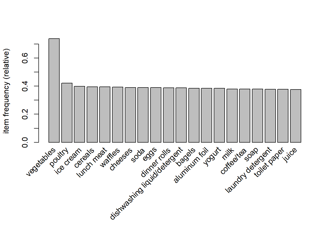
## yogurt} 2- Buscar ayuda de itemFrequencyPlot para visualizar las 20 transacciones más frecuentes.
- Generar las reglas de asociación con 80% de confianza y 15% de soporte.
## Apriori
##
## Parameter specification:
##  confidence minval smax arem  aval originalSupport maxtime support minlen
##         0.5    0.1    1 none FALSE            TRUE       5     0.1      1
##  maxlen target   ext
##      10  rules FALSE
##
## Algorithmic control:
##  filter tree heap memopt load sort verbose
##     0.1 TRUE TRUE  FALSE TRUE    2    TRUE
##
## Absolute minimum support count: 113
##
## set item appearances ...[0 item(s)] done [0.00s].
## set transactions ...[38 item(s), 1139 transaction(s)] done [0.00s].
## sorting and recoding items ... [38 item(s)] done [0.00s].
## creating transaction tree ... done [0.00s].
## checking subsets of size 1 2 3 done [0.00s].
## writing ... [716 rule(s)] done [0.00s].
## creating S4 object ... done [0.00s].- Ver las reglas generadas y ordenalas por lift. Guarda el resultado en una variable nueva.
##     lhs                                          rhs          support
## [1] {soda,vegetables}                         => {eggs}       0.1580334
## [2] {dinner rolls,vegetables}                 => {eggs}       0.1562774
## [3] {pasta,vegetables}                        => {eggs}       0.1439860
## [4] {dishwashing liquid/detergent,vegetables} => {eggs}       0.1536435
## [5] {lunch meat,vegetables}                   => {waffles}    0.1571554
## [6] {individual meals,vegetables}             => {lunch meat} 0.1431080
##     confidence lift     count
## [1] 0.5172414  1.326887 180
## [2] 0.5071225  1.300929 178
## [3] 0.5030675  1.290527 164
## [4] 0.5014327  1.286333 175
## [5] 0.5042254  1.279093 179
## [6] 0.5015385 1.269450 163- Elimina todas las reglas redundantes. Calcula el % de reglas redundantes que había.
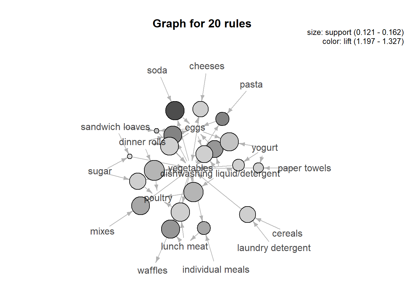
## [1] 11.45251## set of 634 rules- Dibuja las reglas ordenadas y no redundantes usando paquete arulesViz. Si son muchas visualiza las 20 primeras.
##      lhs                                          rhs          support
## [1]  {soda,vegetables}                         => {eggs}       0.1580334
## [2]  {dinner rolls,vegetables}                 => {eggs}       0.1562774
## [3]  {pasta,vegetables}                        => {eggs}       0.1439860
## [4]  {dishwashing liquid/detergent,vegetables} => {eggs}       0.1536435
## [5]  {lunch meat,vegetables}                   => {waffles}    0.1571554
## [6]  {individual meals,vegetables}             => {lunch meat} 0.1431080
## [7]  {mixes,vegetables}                        => {poultry}    0.1562774
## [8]  {dinner rolls,vegetables}                 => {poultry}    0.1615452
## [9]  {dishwashing liquid/detergent,vegetables} => {poultry}    0.1597893
## [10] {eggs,sandwich loaves}                    => {vegetables} 0.1211589
## [11] {eggs,yogurt}                             => {vegetables} 0.1571554
## [12] {dinner rolls,eggs}                       => {vegetables} 0.1562774
## [13] {dishwashing liquid/detergent,eggs}       => {vegetables} 0.1536435
## [14] {sugar,vegetables}                        => {poultry}    0.1518876
## [15] {cereals,laundry detergent}               => {vegetables} 0.1510097
## [16] {paper towels,yogurt}                     => {vegetables} 0.1352063
## [17] {lunch meat,vegetables}                   => {poultry}    0.1580334
## [18] {dishwashing liquid/detergent,yogurt}     => {vegetables} 0.1404741
## [19] {cheeses,eggs}                            => {vegetables} 0.1501317
## [20] {sandwich loaves,sugar}                   => {vegetables} 0.1211589
##      confidence lift     count
## [1]  0.5172414  1.326887 180
## [2]  0.5071225  1.300929 178
## [3]  0.5030675  1.290527 164
## [4]  0.5014327  1.286333 175
## [5]  0.5042254  1.279093 179
## [6]  0.5015385  1.269450 163
## [7]  0.5281899  1.253351 178
## [8]  0.5242165  1.243922 184
## [9]  0.5214900  1.237452 182
## [10] 0.9019608  1.220111 138
## [11] 0.8994975  1.216779 179
## [12] 0.8989899  1.216092 178
## [13] 0.8974359  1.213990 175
## [14] 0.5103245  1.210957 173
## [15] 0.8911917  1.205543 172
## [16] 0.8901734  1.204166 154
## [17] 0.5070423  1.203169 180
## [18] 0.8888889  1.202428 160
## [19] 0.8860104  1.198534 171
## [20] 0.8846154  1.196647 138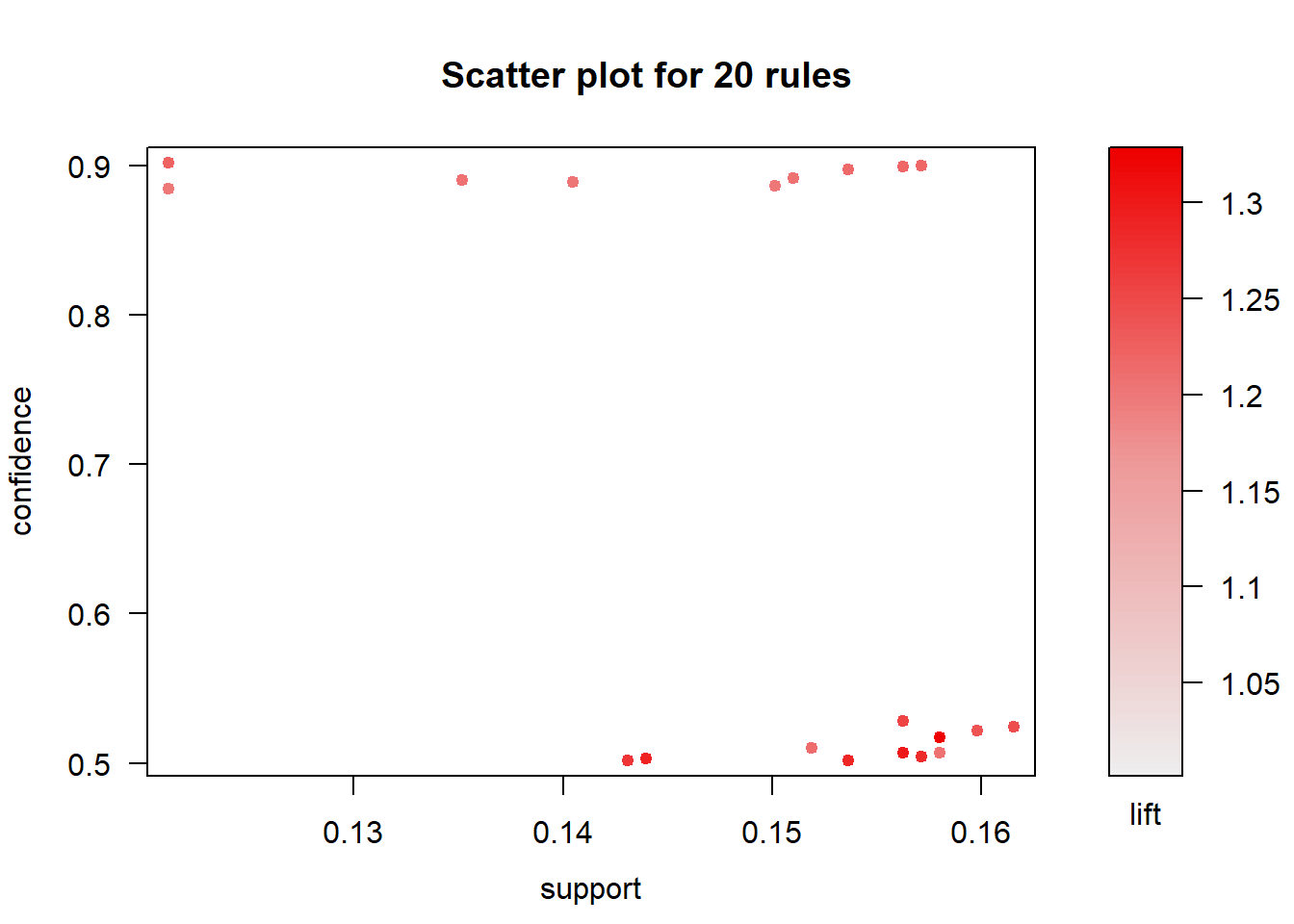
## Itemsets in Antecedent (LHS)
##  [1] "{soda,vegetables}"
##  [2] "{pasta,vegetables}"
##  [3] "{dinner rolls,vegetables}"
##  [4] "{individual meals,vegetables}"
##  [5] "{dishwashing liquid/detergent,vegetables}"
##  [6] "{mixes,vegetables}"
##  [7] "{lunch meat,vegetables}"
##  [8] "{eggs,sandwich loaves}"
##  [9] "{eggs,yogurt}"
## [10] "{dinner rolls,eggs}"
## [11] "{dishwashing liquid/detergent,eggs}"
## [12] "{sugar,vegetables}"
## [13] "{cereals,laundry detergent}"
## [14] "{paper towels,yogurt}"
## [15] "{dishwashing liquid/detergent,yogurt}"
## [16] "{cheeses,eggs}"
## [17] "{sandwich loaves,sugar}"
## Itemsets in Consequent (RHS)
## [1] "{vegetables}" "{poultry}"    "{lunch meat}" "{waffles}"    "{eggs}"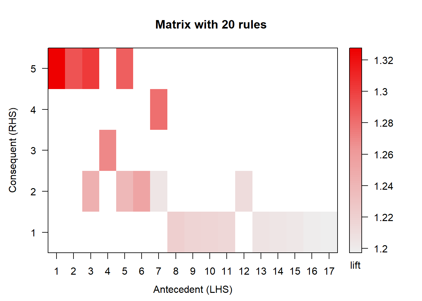
## Itemsets in Antecedent (LHS)
##  [1] "{soda,vegetables}"
##  [2] "{dinner rolls,vegetables}"
##  [3] "{pasta,vegetables}"
##  [4] "{dishwashing liquid/detergent,vegetables}"
##  [5] "{lunch meat,vegetables}"
##  [6] "{individual meals,vegetables}"
##  [7] "{mixes,vegetables}"
##  [8] "{eggs,sandwich loaves}"
##  [9] "{eggs,yogurt}"
## [10] "{dinner rolls,eggs}"
## [11] "{dishwashing liquid/detergent,eggs}"
## [12] "{sugar,vegetables}"
## [13] "{cereals,laundry detergent}"
## [14] "{paper towels,yogurt}"
## [15] "{dishwashing liquid/detergent,yogurt}"
## [16] "{cheeses,eggs}"
## [17] "{sandwich loaves,sugar}"
## Itemsets in Consequent (RHS)
## [1] "{eggs}"       "{waffles}"    "{lunch meat}" "{poultry}"    "{vegetables}"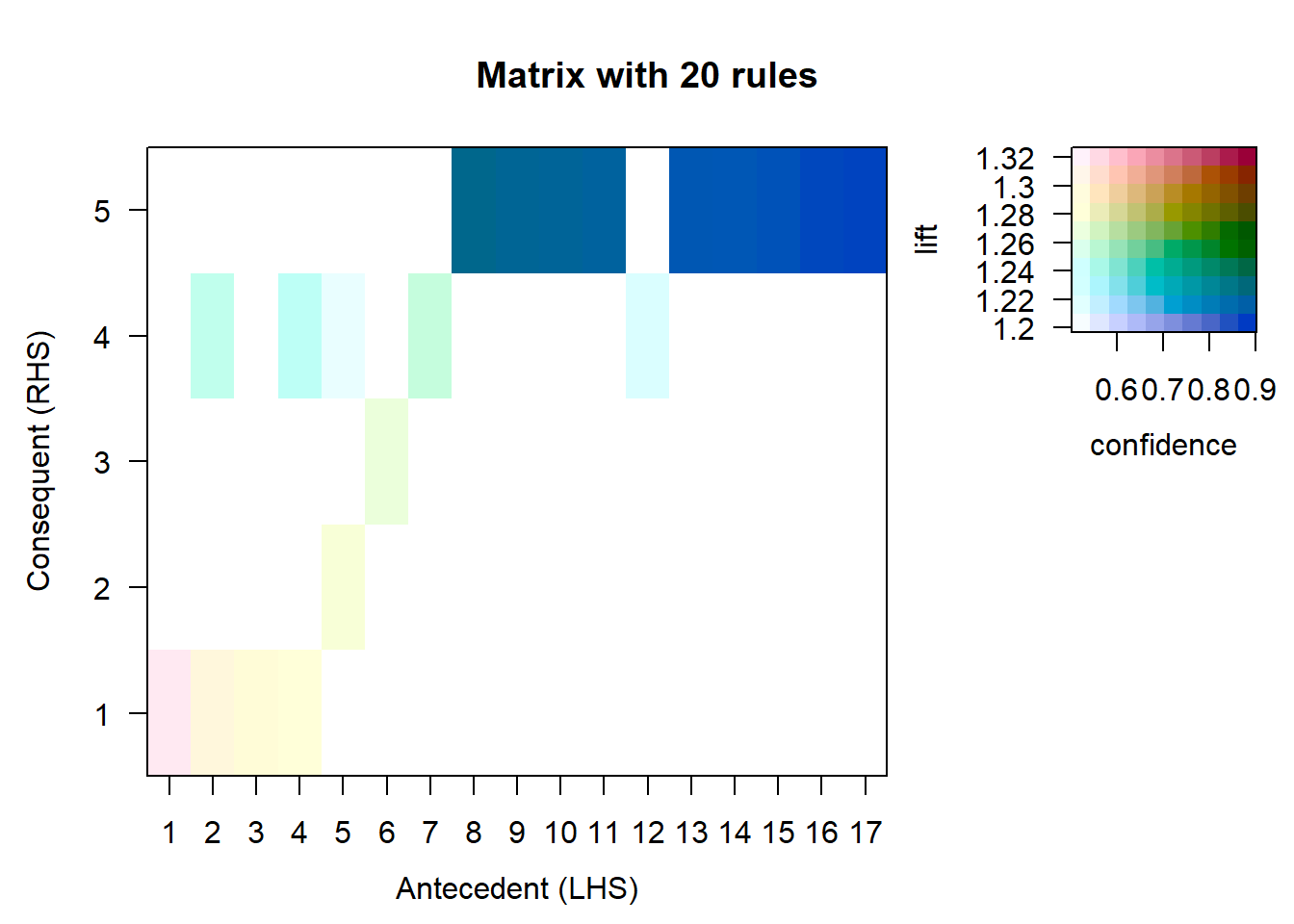
## Loading required namespace: Rgraphviz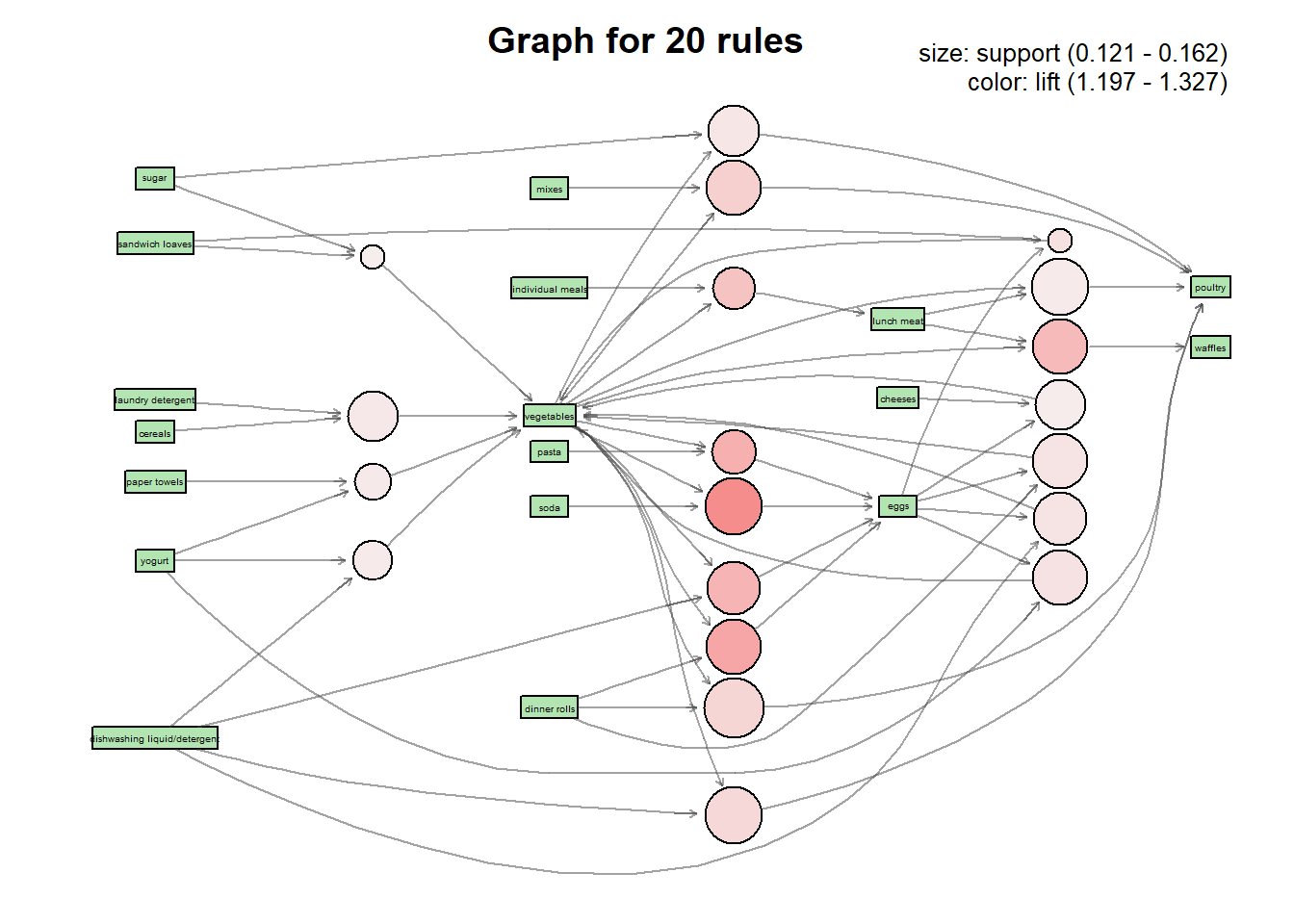
# Visualizacion interactiva
# plot(subrules, method="graph", engine="htmlwidget")
# plot(subrules, method="graph", engine="htmlwidget", igraphLayout = "layout_in_circle")
4.2 FCA
4.2.1 Introduccion a FCA (formal Concept Analysis)
Formal Concept Analysis es un método de análisis de datos, el cuál describe la relación entre un conjunto particular de objetos y un conjunto particular de atributos. FCA genera dos tipos de salidas o ejecuciones a partir de los datos de entrada.
El primer tipo de salida es un retículo de conceptos, el cuál es una colección de conceptos formales que son ordenados jerarquicamente por la relación subconcepto y superconcepto (Al igual que en álgebra hablamos de infimos y supremos).
El segundo tipo de salida consiste en formulas, llamadas implicaciones de atributo, las cuales describen dependencias de atributos concretos que son TRUE en la tabla de datos.
Estas definiciones pertencen a los apuntes de Gerd Stumme suministrados en el campus.
FCA models concepts as units of thought, consisting of two parts:
- The extension consists of all objects belonging to the concept.
- The intension consists of all attributes common to all those objects.
FCA is used for data analysis, information retrieval, and knowledge discovery.
FCA can be understood as conceptual clustering method, which clusters simultanously objects and their descriptions.
FCA can also be used for efficiently computing association rules.
4.2.2 Ejercicio fcaR - tutorialGanter - 1ra parte
- Importar el dataset contextformal_tutorialGanter.csv que se encuentra en CV en variable dataset_ganter
- Los nombres de las filas te aparece como primera columna. Si esto es así, traslada el nombre de las filas a la variable rownames(dataset_ganter)
rownames(dataset_ganter) <- dataset_ganter[,1]
# Eliminamos la primera columna
dataset_ganter <- dataset_ganter[,-1]- Introduce el dataset anterior en un contexto formal de nombre fc_ganter usando el paquete fcaR Imprime el contexto formal (print). Haz plot también del contexto formal.
## Warning: Too many attributes, output will be truncated.## FormalContext with 7 objects and 9 attributes.
## Attributes' names are: needs.water, lives.in.water, lives.on.hand,
## needs.chlorophyll, two.seeds.leaves, one.seed.leaf, ...
## Matrix:
## needs.water lives.in.water lives.on.hand needs.chlorophyll
## Leech 1 1 0 0
## Bream 1 1 0 0
## Frog 1 1 1 0
## Spike-Weed 1 1 0 1
## Reed 1 1 1 1
## Bean 1 0 1 1
## two.seeds.leaves one.seed.leaf can.move.around
## Leech 0 0 1
## Bream 0 0 1
## Frog 0 0 1
## Spike-Weed 0 1 0
## Reed 0 1 0
## Bean 1 0 0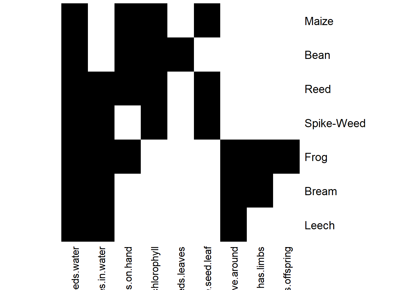
- Convierte a latex el contexto formal. En el Rmd introduce el código latex del contexto formal para visualizarlo.
## \begin{table} \centering
## \begin{tabular}{lrrrrrrrrr}
## \toprule
##   & needs.water & lives.in.water & lives.on.hand & needs.chlorophyll & two.seeds.leaves & one.seed.leaf & can.move.around & has.limbs & suckles.its.offspring\\
## \midrule
## Leech & 1 & 1 & 0 & 0 & 0 & 0 & 1 & 0 & 0\\
## Bream & 1 & 1 & 0 & 0 & 0 & 0 & 1 & 1 & 0\\
## Frog & 1 & 1 & 1 & 0 & 0 & 0 & 1 & 1 & 1\\
## Spike-Weed & 1 & 1 & 0 & 1 & 0 & 1 & 0 & 0 & 0\\
## Reed & 1 & 1 & 1 & 1 & 0 & 1 & 0 & 0 & 0\\
## Bean & 1 & 0 & 1 & 1 & 1 & 0 & 0 & 0 & 0\\
## Maize & 1 & 0 & 1 & 1 & 0 & 1 & 0 & 0 & 0\\
## \bottomrule
## \end{tabular} \caption{\label{}} \end{table}- Guarda todos los atributos en una variable attr_ganter usando los comandos del paquete fcaR. Guarda todos los objetos en una variable obj_ganter usando los comandos del paquete fcaR.
- ¿De que tipo es la variable attr_ganter?
## [1] "character"## chr [1:9] "needs.water" "lives.in.water" "lives.on.hand" ...- ¿De que tipo es la variable attr_objetos?
## [1] "character"## chr [1:7] "Leech" "Bream" "Frog" "Spike-Weed" "Reed" "Bean" "Maize"- Visualizando el contexto formal y utilizando los operadores de derivación, calcula dos conceptos sin usar el método que calcula todos los conceptos.
# Definimos un set de objetos
S <- SparseSet$new(attributes = fc_ganter$objects)
S$assign(Frog = 1) # Asignamos 1 al objeto frog
S
## {Frog}# Computamos el intent del conjunto, obteniendo los atributos que cumple el objeto frog
fc_ganter$intent(S)## {needs.water, lives.in.water, lives.on.hand, can.move.around, has.limbs,
## suckles.its.offspring}# Definimos un set de atributos
D <- SparseSet$new(attributes = fc_ganter$attributes)
D$assign(needs.water = 1, lives.in.water = 1) # Asignamos 1 a los atributos especificados
D## {needs.water, lives.in.water}# Calculamos el extent del conjunto, obteniendo los objetos que poseen dichas propiedades
fc_ganter$extent(D)## {Leech, Bream, Frog, Spike-Weed, Reed}- Usar método de fcaR para calcular todos los conceptos.
# Hacemos uso de la funcion find_implications, la cual extrae las bases canónicas de las implicaciones y el reticulo de conceptos
fc_ganter$find_implications()- ¿Cuantos conceptos hemos calculado a partir del contexto formal?
## [1] 15- Muestra los 10 primeros conceptos.
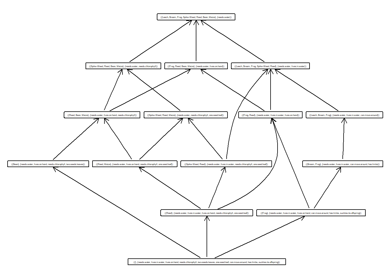
## ({Leech, Bream, Frog, Spike-Weed, Reed, Bean, Maize}, {needs.water})
## ({Spike-Weed, Reed, Bean, Maize}, {needs.water, needs.chlorophyll})
## ({Spike-Weed, Reed, Maize}, {needs.water, needs.chlorophyll, one.seed.leaf})
## ({Frog, Reed, Bean, Maize}, {needs.water, lives.on.hand})
## ({Reed, Bean, Maize}, {needs.water, lives.on.hand, needs.chlorophyll})
## ({Reed, Maize}, {needs.water, lives.on.hand, needs.chlorophyll, one.seed.leaf})
## ({Bean}, {needs.water, lives.on.hand, needs.chlorophyll, two.seeds.leaves})
## ({Leech, Bream, Frog, Spike-Weed, Reed}, {needs.water, lives.in.water})
## ({Leech, Bream, Frog}, {needs.water, lives.in.water, can.move.around})
## ({Bream, Frog}, {needs.water, lives.in.water, can.move.around, has.limbs})- Dibuja el retículo de conceptos
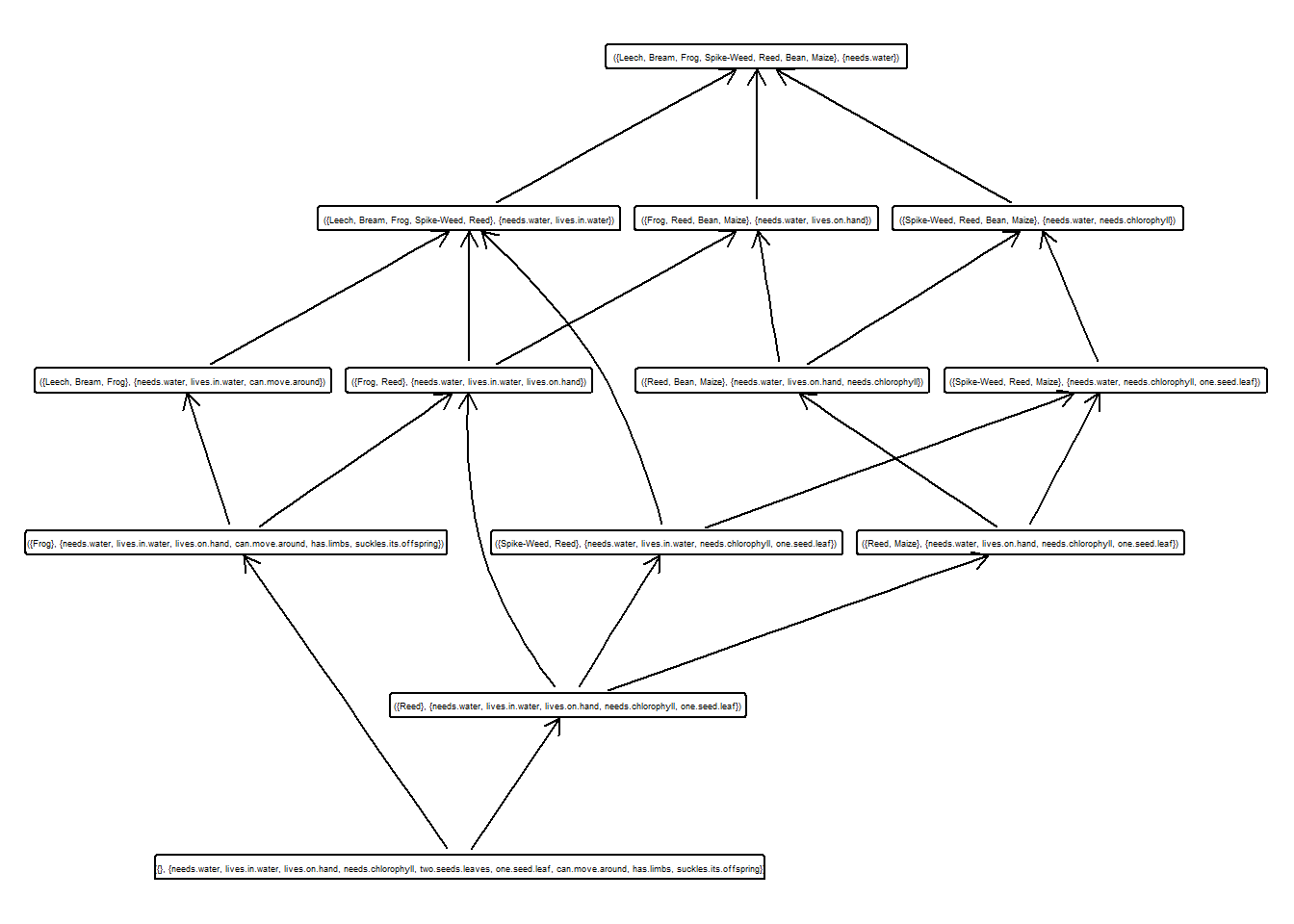
- Calcular y guardar en una variable el subretículo con soporte mayor que 0.3.
idx <- which(fc_ganter$concepts$support() > 0.3)
sublattice <- fc_ganter$concepts$sublattice(idx)
sublattice
## A set of 13 concepts:
## 1: ({Leech, Bream, Frog, Spike-Weed, Reed, Bean, Maize}, {needs.water})
## 2: ({Spike-Weed, Reed, Bean, Maize}, {needs.water, needs.chlorophyll})
## 3: ({Spike-Weed, Reed, Maize}, {needs.water, needs.chlorophyll, one.seed.leaf})
## 4: ({Frog, Reed, Bean, Maize}, {needs.water, lives.on.hand})
## 5: ({Reed, Bean, Maize}, {needs.water, lives.on.hand, needs.chlorophyll})
## 6: ({Reed, Maize}, {needs.water, lives.on.hand, needs.chlorophyll, one.seed.leaf})
## 7: ({Leech, Bream, Frog, Spike-Weed, Reed}, {needs.water, lives.in.water})
## 8: ({Leech, Bream, Frog}, {needs.water, lives.in.water, can.move.around})
## 9: ({Spike-Weed, Reed}, {needs.water, lives.in.water, needs.chlorophyll, one.seed.leaf})
## 10: ({Frog, Reed}, {needs.water, lives.in.water, lives.on.hand})
## 11: ({Frog}, {needs.water, lives.in.water, lives.on.hand, can.move.around, has.limbs, suckles.its.offspring})
## 12: ({Reed}, {needs.water, lives.in.water, lives.on.hand, needs.chlorophyll, one.seed.leaf})
## 13: ({}, {needs.water, lives.in.water, lives.on.hand, needs.chlorophyll, two.seeds.leaves, one.seed.leaf, can.move.around, has.limbs, suckles.its.offspring})- Dibujar dicho subretículo
- ¿De que tipo es el subretículo obtenido?
## [1] "ConceptLattice" "R6"- ¿Qué metodos puedes usar con el subretículo calculado? Pon ejemplos y explica.
# clone --> Los objetos del tipo reticulo son clonables haciendo uso de este metodo
# extents --> Devuelve los extent de todos los conceptos en forma de dgCMatrix
sublattice$extents()
## 7 x 13 sparse Matrix of class "dgCMatrix"
##
## [1,] 1 . . . . . 1 1 . . . . .
## [2,] 1 . . . . . 1 1 . . . . .
## [3,] 1 . . 1 . . 1 1 . 1 1 . .
## [4,] 1 1 1 . . . 1 . 1 . . . .
## [5,] 1 1 1 1 1 1 1 . 1 1 . 1 .
## [6,] 1 1 . 1 1 . . . . . . . .
## [7,] 1 1 1 1 1 1 . . . . . . .# infimum --> Devuelve el infimo de la lista de conceptos que se pase como argumento
# intents --> Devuelve los intents de todos los conceptos en forma de dgCMAtrix
sublattice$intents()## 9 x 13 sparse Matrix of class "dgCMatrix"
##
## [1,] 1 1 1 1 1 1 1 1 1 1 1 1 1
## [2,] . . . . . . 1 1 1 1 1 1 1
## [3,] . . . 1 1 1 . . . 1 1 1 1
## [4,] . 1 1 . 1 1 . . 1 . . 1 1
## [5,] . . . . . . . . . . . . 1
## [6,] . . 1 . . 1 . . 1 . . 1 1
## [7,] . . . . . . . 1 . . 1 . 1
## [8,] . . . . . . . . . . 1 . 1
## [9,] . . . . . . . . . . 1 . 1# is_empty --> Devuelve un booleano al comprobar si el reticulo tiene o no conceptos
sublattice$is_empty()## [1] FALSE# join_irreducibles --> Devuelve los elementos join-irreducibles del reticulo
sublattice$join_irreducibles()## ({Reed, Bean, Maize}, {needs.water, lives.on.hand, needs.chlorophyll})
## ({Reed, Maize}, {needs.water, lives.on.hand, needs.chlorophyll, one.seed.leaf})
## ({Leech, Bream, Frog}, {needs.water, lives.in.water, can.move.around})
## ({Spike-Weed, Reed}, {needs.water, lives.in.water, needs.chlorophyll, one.seed.leaf})
## ({Frog}, {needs.water, lives.in.water, lives.on.hand, can.move.around, has.limbs,
## suckles.its.offspring})
## ({Reed}, {needs.water, lives.in.water, lives.on.hand, needs.chlorophyll,
## one.seed.leaf})# lower_neighbours --> Devuelve una lista con los vecinos inferiores del concepto que se pase como argumento
sublattice$lower_neighbours(sublattice[2])## ({Spike-Weed, Reed, Maize}, {needs.water, needs.chlorophyll, one.seed.leaf})
## ({Reed, Bean, Maize}, {needs.water, lives.on.hand, needs.chlorophyll})# meet_irreducibles --> Devuelve los elementos meet-irreducibles del reticulo
sublattice$meet_irreducibles()## ({Spike-Weed, Reed, Bean, Maize}, {needs.water, needs.chlorophyll})
## ({Spike-Weed, Reed, Maize}, {needs.water, needs.chlorophyll, one.seed.leaf})
## ({Frog, Reed, Bean, Maize}, {needs.water, lives.on.hand})
## ({Leech, Bream, Frog, Spike-Weed, Reed}, {needs.water, lives.in.water})
## ({Leech, Bream, Frog}, {needs.water, lives.in.water, can.move.around})# plot --> Para representar el reticulo
# print --> Para imprimir el contexto formal
sublattice$print()## A set of 13 concepts:
## 1: ({Leech, Bream, Frog, Spike-Weed, Reed, Bean, Maize}, {needs.water})
## 2: ({Spike-Weed, Reed, Bean, Maize}, {needs.water, needs.chlorophyll})
## 3: ({Spike-Weed, Reed, Maize}, {needs.water, needs.chlorophyll, one.seed.leaf})
## 4: ({Frog, Reed, Bean, Maize}, {needs.water, lives.on.hand})
## 5: ({Reed, Bean, Maize}, {needs.water, lives.on.hand, needs.chlorophyll})
## 6: ({Reed, Maize}, {needs.water, lives.on.hand, needs.chlorophyll, one.seed.leaf})
## 7: ({Leech, Bream, Frog, Spike-Weed, Reed}, {needs.water, lives.in.water})
## 8: ({Leech, Bream, Frog}, {needs.water, lives.in.water, can.move.around})
## 9: ({Spike-Weed, Reed}, {needs.water, lives.in.water, needs.chlorophyll, one.seed.leaf})
## 10: ({Frog, Reed}, {needs.water, lives.in.water, lives.on.hand})
## 11: ({Frog}, {needs.water, lives.in.water, lives.on.hand, can.move.around, has.limbs, suckles.its.offspring})
## 12: ({Reed}, {needs.water, lives.in.water, lives.on.hand, needs.chlorophyll, one.seed.leaf})
## 13: ({}, {needs.water, lives.in.water, lives.on.hand, needs.chlorophyll, two.seeds.leaves, one.seed.leaf, can.move.around, has.limbs, suckles.its.offspring})## [1] 13# subconcepts --> Podemos calcular subconceptos de un concepto que se le pase como argumento
sublattice$subconcepts(sublattice[2])## ({Spike-Weed, Reed, Bean, Maize}, {needs.water, needs.chlorophyll})
## ({Spike-Weed, Reed, Maize}, {needs.water, needs.chlorophyll, one.seed.leaf})
## ({Reed, Bean, Maize}, {needs.water, lives.on.hand, needs.chlorophyll})
## ({Reed, Maize}, {needs.water, lives.on.hand, needs.chlorophyll, one.seed.leaf})
## ({Spike-Weed, Reed}, {needs.water, lives.in.water, needs.chlorophyll, one.seed.leaf})
## ({Reed}, {needs.water, lives.in.water, lives.on.hand, needs.chlorophyll,
## one.seed.leaf})
## ({}, {needs.water, lives.in.water, lives.on.hand, needs.chlorophyll,
## two.seeds.leaves, one.seed.leaf, can.move.around, has.limbs,
## suckles.its.offspring})# sublattice --> Podemos obtener un nuevo subreticulo a partir del actual
# superconcepts --> Devuelve una lista con los superconceptos
sublattice$superconcepts(sublattice[2])## ({Leech, Bream, Frog, Spike-Weed, Reed, Bean, Maize}, {needs.water})
## ({Spike-Weed, Reed, Bean, Maize}, {needs.water, needs.chlorophyll})## [1] 1.0000000 0.5714286 0.4285714 0.5714286 0.4285714 0.2857143 0.7142857
## [8] 0.4285714 0.2857143 0.2857143 0.1428571 0.1428571 0.0000000# supremum --> Devuelve el supremo de la lista de conceptos que se pase como argumento
# to_latex --> Convertir el contexto formal en codigo latex
sublattice$to_latex()## \begin{longtable}{lll}
## 1: &$\left(\,\ensuremath{\{Leech,\, Bream,\, Frog,\, Spike-Weed,\, Reed,\, Bean,\, Maize\}},\right.$&$\left.\ensuremath{\{needs.water\}}\,\right)$\\
## 2: &$\left(\,\ensuremath{\{Spike-Weed,\, Reed,\, Bean,\, Maize\}},\right.$&$\left.\ensuremath{\{needs.water,\, needs.chlorophyll\}}\,\right)$\\
## 3: &$\left(\,\ensuremath{\{Spike-Weed,\, Reed,\, Maize\}},\right.$&$\left.\ensuremath{\{needs.water,\, needs.chlorophyll,\, one.seed.leaf\}}\,\right)$\\
## 4: &$\left(\,\ensuremath{\{Frog,\, Reed,\, Bean,\, Maize\}},\right.$&$\left.\ensuremath{\{needs.water,\, lives.on.hand\}}\,\right)$\\
## 5: &$\left(\,\ensuremath{\{Reed,\, Bean,\, Maize\}},\right.$&$\left.\ensuremath{\{needs.water,\, lives.on.hand,\, needs.chlorophyll\}}\,\right)$\\
## 6: &$\left(\,\ensuremath{\{Reed,\, Maize\}},\right.$&$\left.\ensuremath{\{needs.water,\, lives.on.hand,\, needs.chlorophyll,\, one.seed.leaf\}}\,\right)$\\
## 7: &$\left(\,\ensuremath{\{Leech,\, Bream,\, Frog,\, Spike-Weed,\, Reed\}},\right.$&$\left.\ensuremath{\{needs.water,\, lives.in.water\}}\,\right)$\\
## 8: &$\left(\,\ensuremath{\{Leech,\, Bream,\, Frog\}},\right.$&$\left.\ensuremath{\{needs.water,\, lives.in.water,\, can.move.around\}}\,\right)$\\
## 9: &$\left(\,\ensuremath{\{Spike-Weed,\, Reed\}},\right.$&$\left.\ensuremath{\{needs.water,\, lives.in.water,\, needs.chlorophyll,\, one.seed.leaf\}}\,\right)$\\
## 10: &$\left(\,\ensuremath{\{Frog,\, Reed\}},\right.$&$\left.\ensuremath{\{needs.water,\, lives.in.water,\, lives.on.hand\}}\,\right)$\\
## 11: &$\left(\,\ensuremath{\{Frog\}},\right.$&$\left.\ensuremath{\{needs.water,\, lives.in.water,\, lives.on.hand,\, can.move.around,\, has.limbs,\, suckles.its.offspring\}}\,\right)$\\
## 12: &$\left(\,\ensuremath{\{Reed\}},\right.$&$\left.\ensuremath{\{needs.water,\, lives.in.water,\, lives.on.hand,\, needs.chlorophyll,\, one.seed.leaf\}}\,\right)$\\
## 13: &$\left(\,\ensuremath{\varnothing},\right.$&$\left.\ensuremath{\{needs.water,\, lives.in.water,\, lives.on.hand,\, needs.chlorophyll,\, two.seeds.leaves,\, one.seed.leaf,\, can.move.around,\, has.limbs,\, suckles.its.offspring\}}\,\right)$\\
## \end{longtable}# upper_neighbours --> Devuelve una lista con los vecinos superiores del concepto que se pase como argumento
sublattice$upper_neighbours(sublattice[2])## ({Leech, Bream, Frog, Spike-Weed, Reed, Bean, Maize}, {needs.water})Para hacer luego con más tiempo: busca información en los tutoriales, o en internet acerca de la definición de soporte de un concepto.
Calcula el superior y el infimo de los conceptos calculados para fc_ganter y lo mismo para el subretículo anterior. Visualizalos.
## ({Bream, Frog}, {needs.water, lives.in.water, can.move.around, has.limbs})
## ({Spike-Weed, Reed}, {needs.water, lives.in.water, needs.chlorophyll, one.seed.leaf})
## ({Frog, Reed}, {needs.water, lives.in.water, lives.on.hand})## ({Leech, Bream, Frog, Spike-Weed, Reed}, {needs.water, lives.in.water})## ({}, {needs.water, lives.in.water, lives.on.hand, needs.chlorophyll,
## two.seeds.leaves, one.seed.leaf, can.move.around, has.limbs,
## suckles.its.offspring})## ({Spike-Weed, Reed, Bean, Maize}, {needs.water, needs.chlorophyll})## ({Spike-Weed, Reed, Maize}, {needs.water, needs.chlorophyll, one.seed.leaf})- Grabar el objeto fc_ganter en un fichero fc_ganter.rds.
- Elimina la variable fc_ganter. Carga otra vez en la variable del fichero anterior y comprueba que tenemos toda la información: atributos, conceptos, etc.
Calcula lo siguientes conjuntos usando los métodos del paquete fcaR:
{Bean}′
{livesonland}′
{twoseedleaves}′
{Frog,Maize}′
{needschlorophylltoproducefood,canmovearound}′
{livesinwater,livesonland}′
{needschlorophylltoproducefood,canmovearound}′
## {needs.water, lives.on.hand, needs.chlorophyll, two.seeds.leaves}# {livesonland}′
# En la tabla tenemos lives on hand, en lugar de lives on land
c2 <- SparseSet$new(fc_ganter2$attributes)
c2$assign(lives.on.hand = 1)
fc_ganter2$extent(c2)## {Frog, Reed, Bean, Maize}# {twoseedleaves}′
c3 <- SparseSet$new(fc_ganter2$attributes)
c3$assign(two.seeds.leaves = 1)
fc_ganter2$extent(c3)## {Bean}# {Frog,Maize}′
c4 <- SparseSet$new(fc_ganter2$objects)
c4$assign(Frog = 1, Maize = 1)
fc_ganter2$intent(c4)## {needs.water, lives.on.hand}# {needschlorophylltoproducefood,canmovearound}′
c5 <- SparseSet$new(fc_ganter2$attributes)
c5$assign(needs.chlorophyll = 1, can.move.around = 1)
fc_ganter2$extent(c5)## {}# {livesinwater,livesonland}′
c6 <- SparseSet$new(fc_ganter2$attributes)
c6$assign(lives.in.water = 1, lives.on.hand = 1)
fc_ganter2$extent(c6)## {Frog, Reed}4.2.3 Ejercicio Tutorial Ganter - 2da parte
Segunda parte, clase 06/05/20
- Calcula las implicaciones del contexto
library('fcaR')
library(arules)
# Recueramos los datos de fc_ganter que previamente se habian eliminado
fc_ganter <- FormalContext$new()
fc_ganter$load("fc_ganter.rds")
# Compute implications
fc_ganter$find_implications(verbose = FALSE)- Muestra las implicaciones en pantalla
## Implication set with 10 implications.
## Rule 1: {} -> {needs.water}
## Rule 2: {needs.water, suckles.its.offspring} -> {lives.in.water,
##   lives.on.hand, can.move.around, has.limbs}
## Rule 3: {needs.water, has.limbs} -> {lives.in.water, can.move.around}
## Rule 4: {needs.water, can.move.around} -> {lives.in.water}
## Rule 5: {needs.water, one.seed.leaf} -> {needs.chlorophyll}
## Rule 6: {needs.water, two.seeds.leaves} -> {lives.on.hand,
##   needs.chlorophyll}
## Rule 7: {needs.water, lives.on.hand, needs.chlorophyll,
##   two.seeds.leaves, one.seed.leaf} -> {lives.in.water, can.move.around,
##   has.limbs, suckles.its.offspring}
## Rule 8: {needs.water, lives.in.water, needs.chlorophyll} ->
##   {one.seed.leaf}
## Rule 9: {needs.water, lives.in.water, needs.chlorophyll,
##   one.seed.leaf, can.move.around} -> {lives.on.hand, two.seeds.leaves,
##   has.limbs, suckles.its.offspring}
## Rule 10: {needs.water, lives.in.water, lives.on.hand, can.move.around}
## -> {has.limbs, suckles.its.offspring}- ¿Cuantas implicaciones se han extraido?
## [1] 10- Calcula el tamaño de las implicaciones y la media de la parte y derecha de dichas implicaciones.
## LHS RHS
## 2.7 2.2- Aplica las reglas de la lógica de simplificación. ¿Cuantas implicaciones han aparecido tras aplicar la lógica?
## Processing batch## --> simplification: from 10 to 10 in 0.05 secs.## Batch took 0.05 secs.## [1] 10## Implication set with 10 implications.
## Rule 1: {} -> {needs.water}
## Rule 2: {suckles.its.offspring} -> {lives.in.water, lives.on.hand,
## can.move.around, has.limbs}
## Rule 3: {has.limbs} -> {lives.in.water, can.move.around}
## Rule 4: {can.move.around} -> {lives.in.water}
## Rule 5: {one.seed.leaf} -> {needs.chlorophyll}
## Rule 6: {two.seeds.leaves} -> {lives.on.hand, needs.chlorophyll}
## Rule 7: {two.seeds.leaves, one.seed.leaf} -> {lives.in.water,
## can.move.around, has.limbs, suckles.its.offspring}
## Rule 8: {lives.in.water, needs.chlorophyll} -> {one.seed.leaf}
## Rule 9: {one.seed.leaf, can.move.around} -> {lives.on.hand,
## two.seeds.leaves, has.limbs, suckles.its.offspring}
## Rule 10: {lives.on.hand, can.move.around} -> {has.limbs,
## suckles.its.offspring}- Eliminar la redundancia en el conjunto de implicaciones. ¿Cuantas implicaciones han aparecido tras aplicar la lógica?
fc_ganter$implications$apply_rules(rules = c("composition",
                                             "generalization",
                                             "simplification"), parallelize = FALSE)
## Processing batch## --> composition: from 10 to 10 in 0 secs.## --> generalization: from 10 to 10 in 0.02 secs.## --> simplification: from 10 to 10 in 0.03 secs.## Batch took 0.05 secs.## Implication set with 10 implications.
## Rule 1: {} -> {needs.water}
## Rule 2: {suckles.its.offspring} -> {lives.in.water, lives.on.hand,
## can.move.around, has.limbs}
## Rule 3: {has.limbs} -> {lives.in.water, can.move.around}
## Rule 4: {can.move.around} -> {lives.in.water}
## Rule 5: {one.seed.leaf} -> {needs.chlorophyll}
## Rule 6: {two.seeds.leaves} -> {lives.on.hand, needs.chlorophyll}
## Rule 7: {two.seeds.leaves, one.seed.leaf} -> {lives.in.water,
## can.move.around, has.limbs, suckles.its.offspring}
## Rule 8: {lives.in.water, needs.chlorophyll} -> {one.seed.leaf}
## Rule 9: {one.seed.leaf, can.move.around} -> {lives.on.hand,
## two.seeds.leaves, has.limbs, suckles.its.offspring}
## Rule 10: {lives.on.hand, can.move.around} -> {has.limbs,
## suckles.its.offspring}## [1] 10- Calcular el cierre de los atributos needs.water, one.seed.leaf.
S <- SparseSet$new(attributes = fc_ganter$attributes)
S$assign("needs.water" = 1, "one.seed.leaf"=1)
S
## {needs.water, one.seed.leaf}## $closure
## {needs.water, needs.chlorophyll, one.seed.leaf}- Copia (clona) el conjunto fc_ganter en una variable fc1.
## Warning: Too many attributes, output will be truncated.## FormalContext with 7 objects and 9 attributes.
## Attributes' names are: needs.water, lives.in.water, lives.on.hand,
## needs.chlorophyll, two.seeds.leaves, one.seed.leaf, ...
## Matrix:
## needs.water lives.in.water lives.on.hand needs.chlorophyll
## Leech 1 1 0 0
## Bream 1 1 0 0
## Frog 1 1 1 0
## Spike-Weed 1 1 0 1
## Reed 1 1 1 1
## Bean 1 0 1 1
## two.seeds.leaves one.seed.leaf can.move.around
## Leech 0 0 1
## Bream 0 0 1
## Frog 0 0 1
## Spike-Weed 0 1 0
## Reed 0 1 0
## Bean 1 0 0
- Elimina la implicación que está en la primera posición:
# Este comando elimina la primera, como en arules
fc1$implications <- fc1$implications[-1]
fc1$implications
## Implication set with 9 implications.
## Rule 1: {suckles.its.offspring} -> {lives.in.water, lives.on.hand,
## can.move.around, has.limbs}
## Rule 2: {has.limbs} -> {lives.in.water, can.move.around}
## Rule 3: {can.move.around} -> {lives.in.water}
## Rule 4: {one.seed.leaf} -> {needs.chlorophyll}
## Rule 5: {two.seeds.leaves} -> {lives.on.hand, needs.chlorophyll}
## Rule 6: {two.seeds.leaves, one.seed.leaf} -> {lives.in.water,
## can.move.around, has.limbs, suckles.its.offspring}
## Rule 7: {lives.in.water, needs.chlorophyll} -> {one.seed.leaf}
## Rule 8: {one.seed.leaf, can.move.around} -> {lives.on.hand,
## two.seeds.leaves, has.limbs, suckles.its.offspring}
## Rule 9: {lives.on.hand, can.move.around} -> {has.limbs,
## suckles.its.offspring}- Extrae de todas las implicaciones la que tengan en el lado izquierdo de la implicación el atributo one.seed.leaf.
# Siguiendo las especificaciones del paquete fcaR, el uso de filter es el siguiente
imp <- fc1$implications$filter(lhs = "one.seed.leaf")
imp
## Implication set with 3 implications.
## Rule 1: {one.seed.leaf} -> {needs.chlorophyll}
## Rule 2: {two.seeds.leaves, one.seed.leaf} -> {lives.in.water,
## can.move.around, has.limbs, suckles.its.offspring}
## Rule 3: {one.seed.leaf, can.move.around} -> {lives.on.hand,
## two.seeds.leaves, has.limbs, suckles.its.offspring}- Correccion –> Obtén los atributos que aparezcan en las implicaciones
## [1] "needs.water"           "lives.in.water"        "lives.on.hand"
## [4] "needs.chlorophyll"     "two.seeds.leaves"      "one.seed.leaf"
## [7] "can.move.around" "has.limbs" "suckles.its.offspring"- Calcula el soporte de la implicación 3
## [1] 0.33333334.3 Regresion
4.3.1 Introduccion
- Correlación –> Es una medida del grado de dependencia entre las variables.
- Regresión –> Pretende encontrar un modelo aproximado de la dependencia entre las variables.
Existen diferentes modelos para poder elaborar curvas de regresión, hay que saber elegir la que mejor se adapte a nuestros datos: lineal, cuadrático, exponencial…
Dada una nube de puntos, llamamos vector residuo \(\overrightarrow{e}\) al error cometido por el ajuste elegido.
Existen diversas tecnicas de modelado. Hay dos tipos de tecnicas numericas basicas: Interpolacion y aproximacion (ajuste).
El objetivo es obtener una funcion que se ajuste lo mejor posible a un conjunto de datos (nube de datos) de observaciones, informacion recopilada por sensores, datasets…
El modelo de ajuste más simple es el modelo lineal (lm), conocido como regresion lineal en Machine Learning.
Otros aprendizajes estadisticos mas complejos son generalizacion de las regresion lineal.
Interpolacion lineal
El objetivo es encontrar una funcion de interpolacion tal que: \(\phi(x) = a_0 + a_1f_1(x)\) (La aproximacion mas sencillas ea considerar funciones polinomicas \(f_1(x) = x\))
De la expresion anterior definimos \(a_0\) como el intercept y \(a_1\) como slope.
Regresion lineal en R
El objetivo es:
- Prediccion de observaciones futuras.
- Encontrar relaciones, es decir, funciones entre variables del dataset.
- Describir la estructura de un dataset
A la hora de establecer una regresion lineal haremos uso de la funcion lm, indicando las variables enfrentadas y los datos: lm(Y~X, data = datos), siendo:
- Y es la variable dependiente, la salida.
- X es la variable independiente, el predictor.
- datos es el dataset con los atributos de X e Y
Los valores obtenidos nos permiten establecer o crear la funcion que buscamos. Ejemplo: \(\phi(x) = -1.5+5.6x\), indicando que el valor de Y esperado cuando X vale 0 es de -1.5 y el incremento o pendiente se corresponde con 5.6.
Evaluando el modelo
- ¿Se ajusta el modelo a la nube de puntos? ¿Probando un modelo mas complejo (polinomico)?
- Si la nube de puntos es de tamaño n, la interpolación se puede conseguir con un polinomio de grado n-1.
- Polinomio de alto grado tienden a introducir errores como oscilaciones, coste computacional,…
- Para cada modelo encontrado, hay que calcular los errores producidos, la precision, etc
Tenemos que conocer los siguientes terminos:
- RSE o error estandar residual, el cual es un estimador de la desviacion estandar de \(e_i\). RSE se considera una medida de la falta de adaptacion o ajuste del modelo a los datos, es decir, cuanto mayor sea su valor, menos se ajusta el modelo a los datos.
- Si la prediccion usando el modelo son buenas, concluimos que el modelo se ajusta bien a los datos. En otras palabras, si el modelo de no se ajusta bien a los datos entonces el RSE será grande.
- \(R^2\) (coeficiente de determinacion) toma la forma de una medida de proporcion, es decir, la proporcion de la varianza en la variable del resultado que puede ser explicada por el predictor.
- Un numero cercano a 1 indica que gran parte de la variacion de la respuesta es explicada por la regresion. Un numero cercano a 0 indica que el modelo lineal es erroneo o que el error inherente es alto, o ambos.
- \(R^2 ajustado\). Cuando añadimos mas predictores al modelo, el valor ajustado de \(R^2\) se incrementará solo si las nuevas variables introducidas mejoran el modelo.
Analizando el plot del modelo
Al realizar un plot de nuestro modelo, obtendremos 4 graficas:
Residuals vs Fitted. El primer plot es un gráfico de dispersion entre valores residuales y valores predecidos. R marca los outliers del dataset.
Normal Q-Q. Es una representacion normal de la probabilidad. Como resultado tendremos una linea recta si los errores estan distribuidos siguiendo una noraml. Los outliers se desvian de esa linea.
Scale-Location. Al igual que la primera, debería tener bastante dispersion de los datos, sin patrones identificables.
Residuals vs leverage. Nos indica que puntos tienen mayor influencia en la regresion. Para detectar outliers, eliminamos esos puntos y repetimos el modelo.
4.3.2 Ejercicio Regresion Repaso
##
## Attaching package: 'datarium'
## The following object is masked _by_ '.GlobalEnv':
##
## titanic.raw## youtube facebook newspaper sales
## 1 276.12 45.36 83.04 26.52
## 2 53.40 47.16 54.12 12.48
## 3 20.64 55.08 83.16 11.16
## 4 181.80 49.56 70.20 22.20
## 5 216.96 12.96 70.08 15.48
## 6 10.44 58.68 90.00 8.64El paquete dice las ventas que ha tenido la empresa, la inversion que ha hecho en publicidad, tanto en yt, facebook y periodico. inversion –> ventas
- Analisis exploratorio
## [1] 200 4## 'data.frame': 200 obs. of 4 variables:
## $ youtube : num 276.1 53.4 20.6 181.8 217 ...
## $ facebook : num 45.4 47.2 55.1 49.6 13 ...
## $ newspaper: num 83 54.1 83.2 70.2 70.1 ...
## $ sales : num 26.5 12.5 11.2 22.2 15.5 ...## youtube facebook newspaper sales
## Min. : 0.84 Min. : 0.00 Min. : 0.36 Min. : 1.92
## 1st Qu.: 89.25 1st Qu.:11.97 1st Qu.: 15.30 1st Qu.:12.45
## Median :179.70 Median :27.48 Median : 30.90 Median :15.48
## Mean :176.45 Mean :27.92 Mean : 36.66 Mean :16.83
## 3rd Qu.:262.59 3rd Qu.:43.83 3rd Qu.: 54.12 3rd Qu.:20.88
## Max. :355.68 Max. :59.52 Max. :136.80 Max. :32.40## 0% 25% 50% 75% 100%
## 0.84 89.25 179.70 262.59 355.68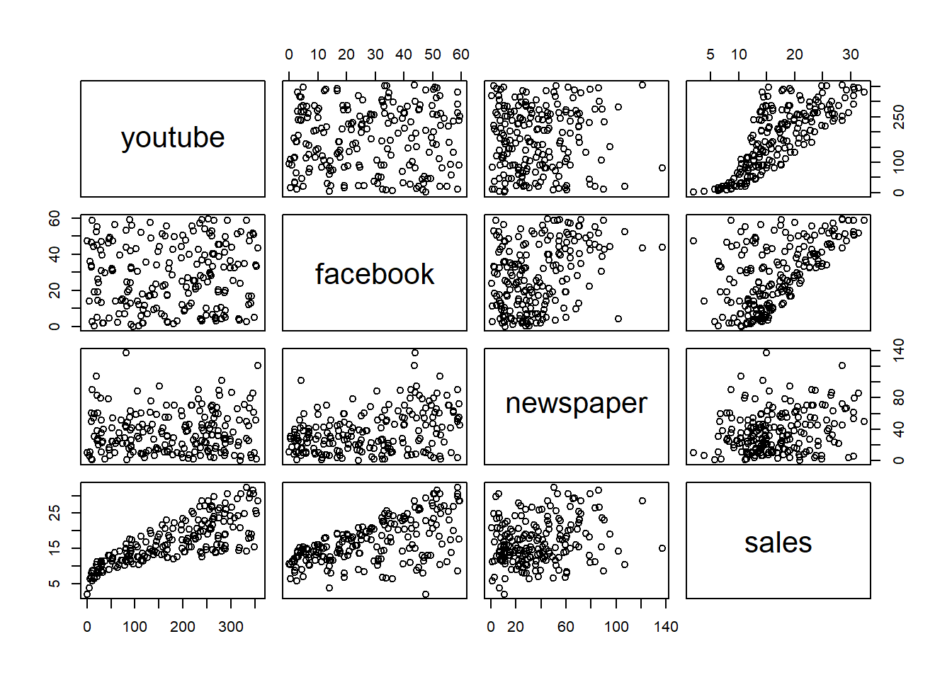
# library(GGally)
# ggpairs(marketing)

p <- marketing %>%
    ggplot(aes(x = youtube, y = sales)) +
    geom_point() +
    stat_smooth()
p
## `geom_smooth()` using method = 'loess' and formula 'y ~ x'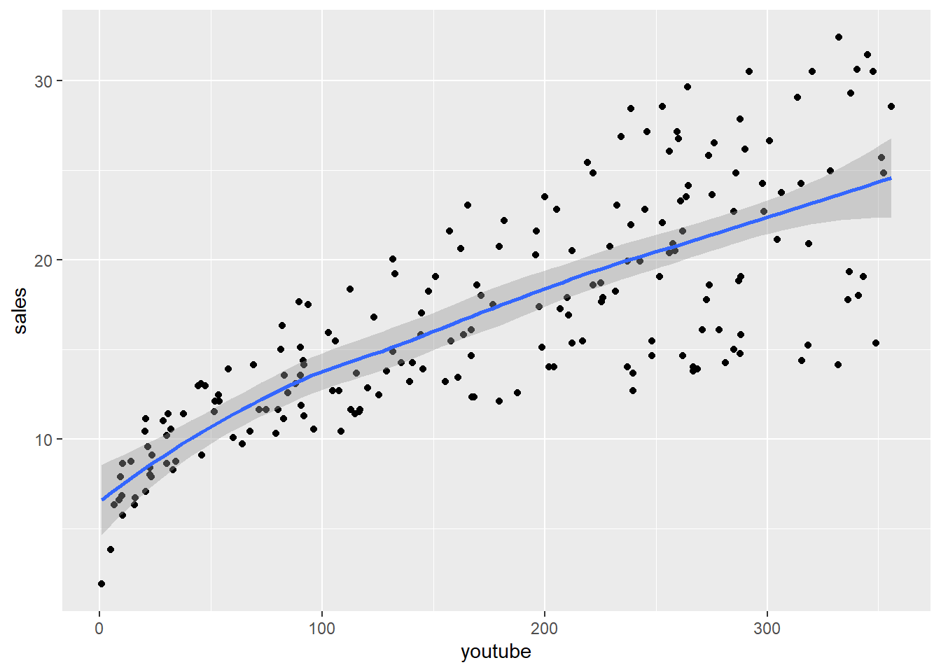
- Gráfico facebook - ventas
## `geom_smooth()` using method = 'loess' and formula 'y ~ x'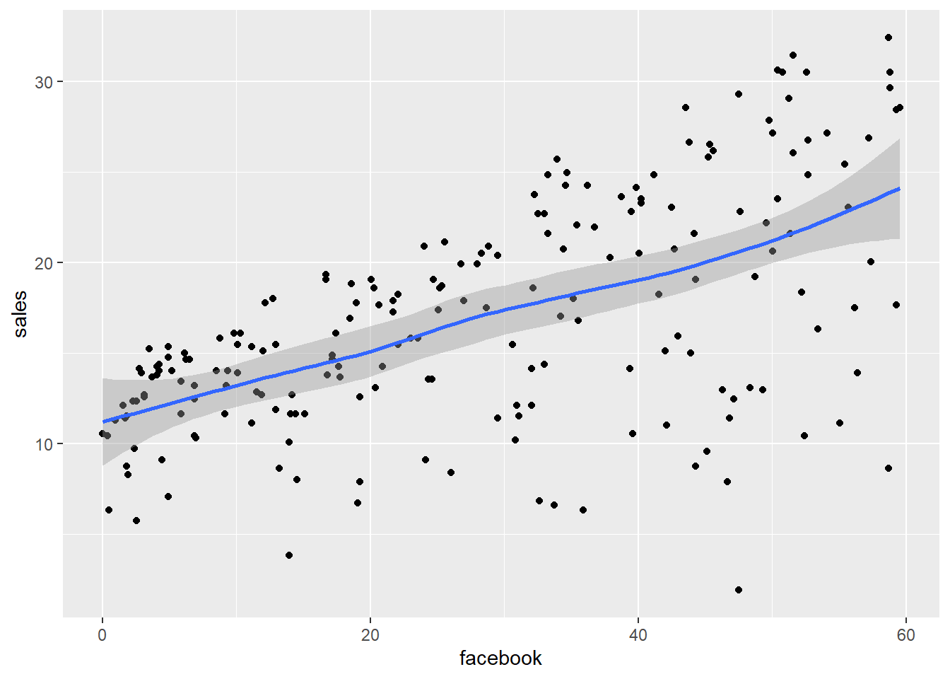
- Gráfico newspaper - ventas
## `geom_smooth()` using method = 'loess' and formula 'y ~ x'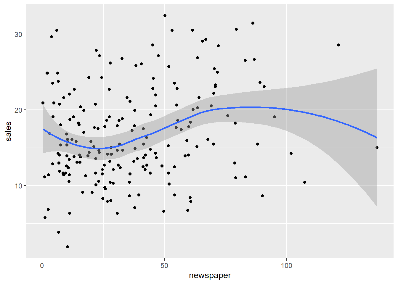
- Correlaciones
## [1] 0.7822244## [1] 0.5762226## [1] 0.228299- Modelo
¿Si hay efecto entre la inversión de las ventas?
# Realizamos modelo de regresion ventas-youtube
ventas_youtube <- lm(sales~youtube, data = marketing)
ventas_youtube
##
## Call:
## lm(formula = sales ~ youtube, data = marketing)
##
## Coefficients:
## (Intercept) youtube
## 8.43911 0.04754ventas = 8.43911 + 0.04754 * youtube
## (Intercept)     youtube
##  8.43911226  0.04753664
# Errores que he cometido en cada punto de mi dataset:
# ventas_youtube$residuals
# Para cada X su Y aproximado:
# ventas_youtube$fitted.values
# Hay mas comandos- Dibujar el modelo y el dataset
# En la Y va la funcion que tu quieres predecir, es decir la ventas
attach(marketing)
# Ejecutar a la vez
plot(youtube, sales)
abline(ventas_youtube)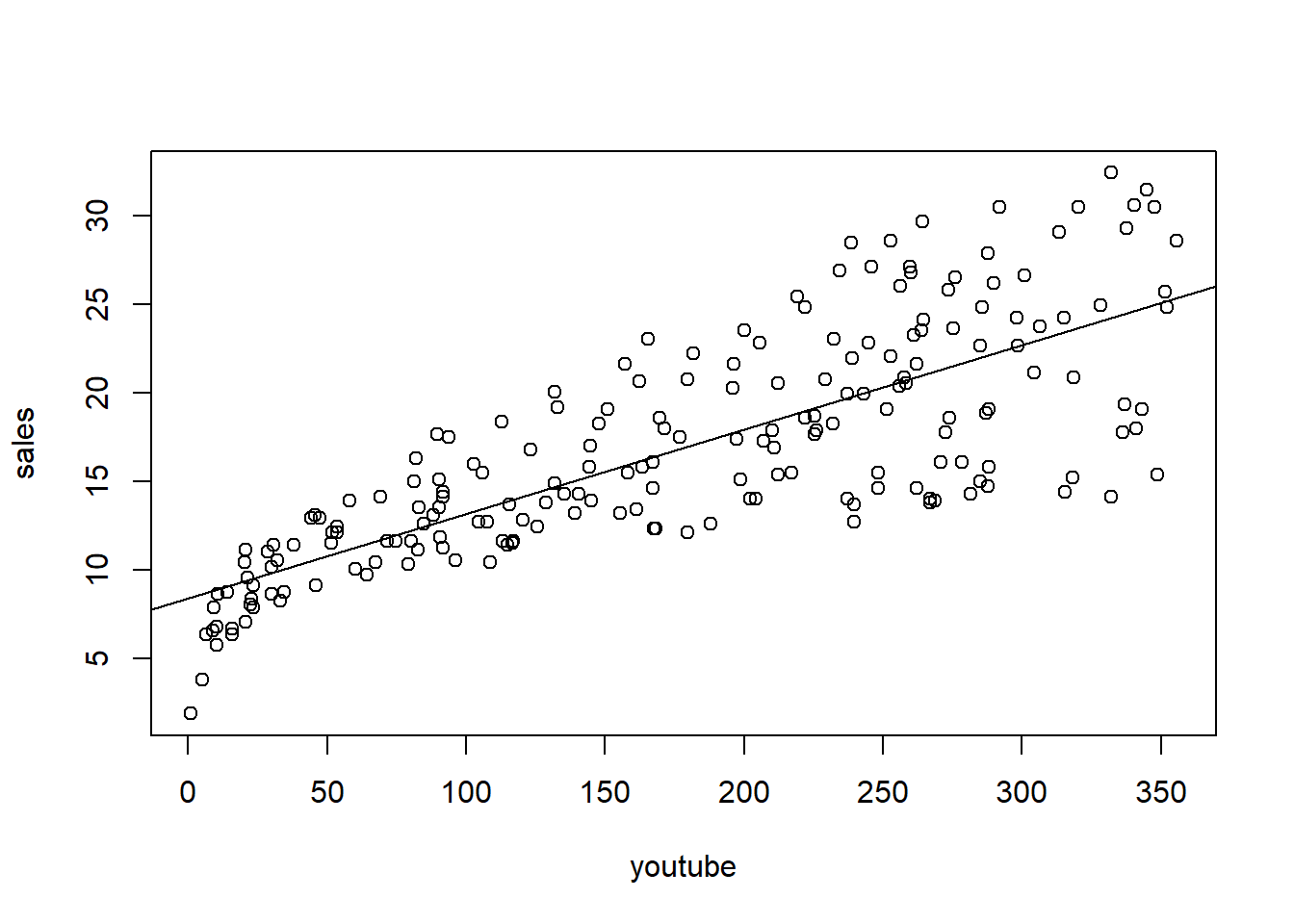
# Usando ggplot
p <- marketing %>%
    ggplot(aes(x = youtube, y = sales)) +
    geom_point() +
    stat_smooth(method = lm)
p
## `geom_smooth()` using formula 'y ~ x'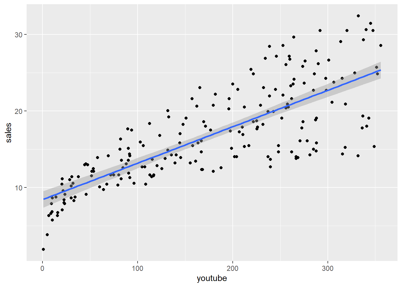
- Plot del modelo
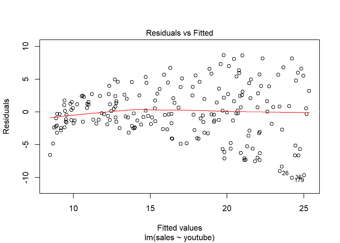
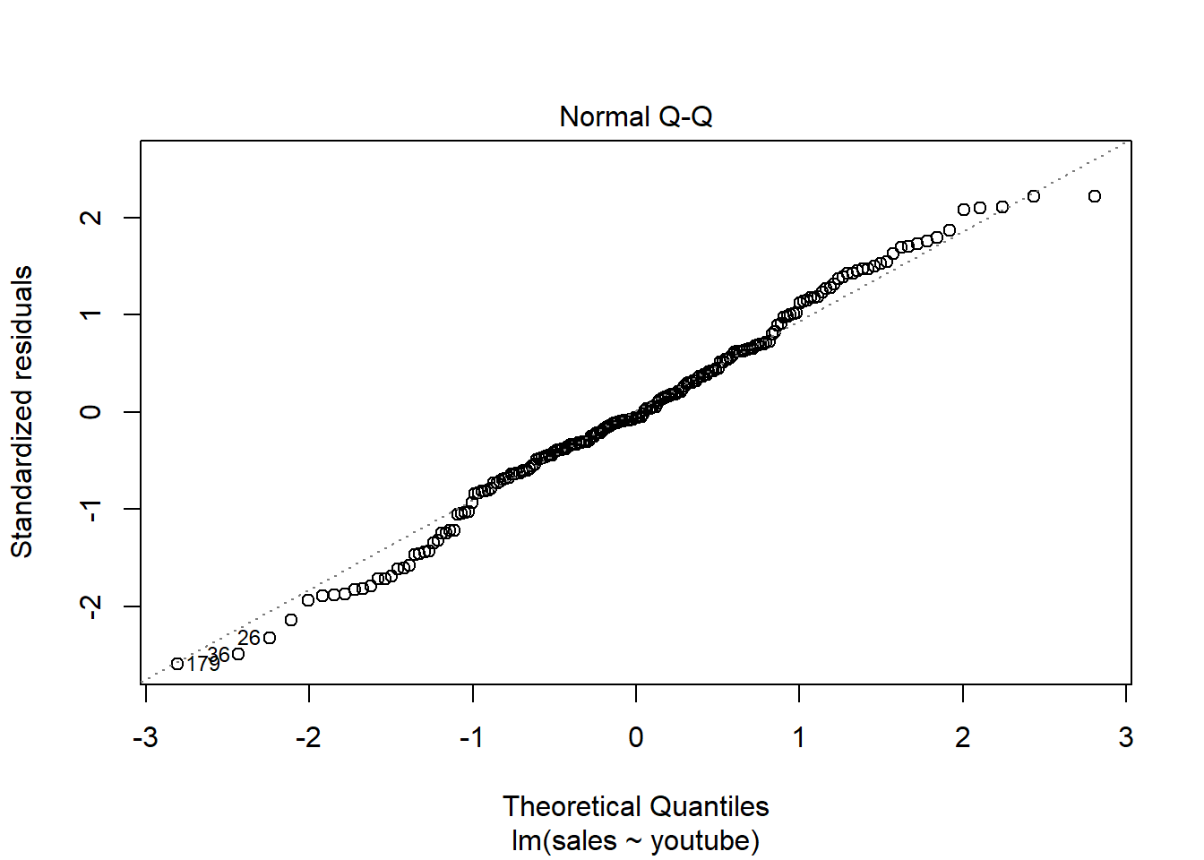
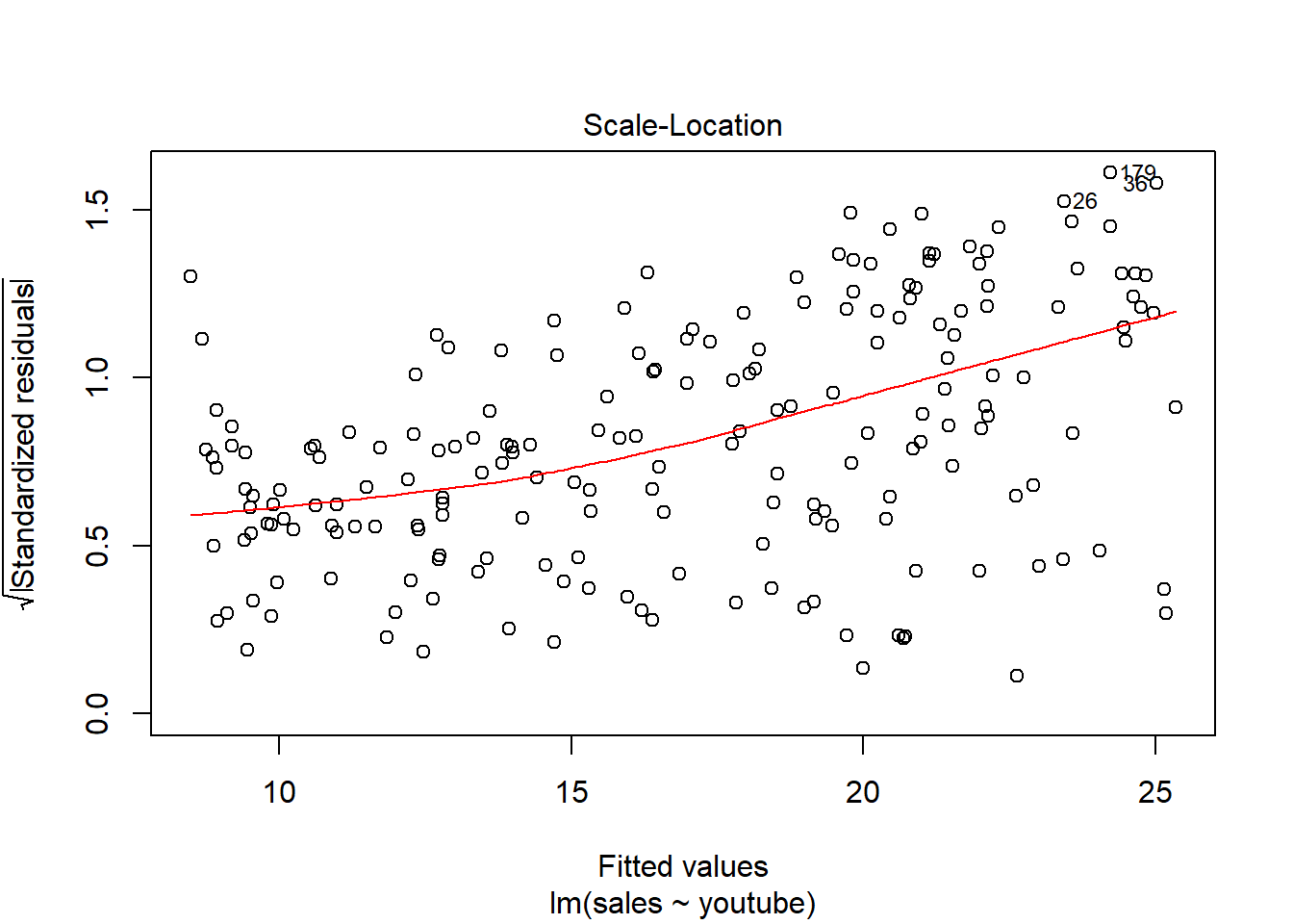
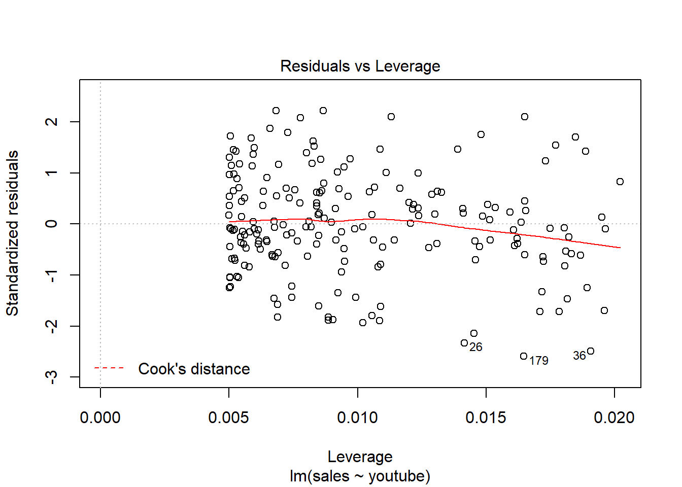
Residuos linealmente distribuidos, cerca del y = 0
Residuos están practicamente distribuidos siguiendo una normal, la y = x. Tambien me detecta outliers, valores importantes usando la distancia de Cook
Residuos están distribuidos aleatoriamente - mucha dispersión de los errores.
Vemos los calculos de la distancia de Cook –> outliers, valores importantes
- Como de bueno es el modelo
##
## Call:
## lm(formula = sales ~ youtube, data = marketing)
##
## Residuals:
## Min 1Q Median 3Q Max
## -10.0632 -2.3454 -0.2295 2.4805 8.6548
##
## Coefficients:
## Estimate Std. Error t value Pr(>|t|)
## (Intercept) 8.439112 0.549412 15.36 <2e-16 ***
## youtube 0.047537 0.002691 17.67 <2e-16 ***
## ---
## Signif. codes: 0 '***' 0.001 '**' 0.01 '*' 0.05 '.' 0.1 ' ' 1
##
## Residual standard error: 3.91 on 198 degrees of freedom
## Multiple R-squared: 0.6119, Adjusted R-squared: 0.6099
## F-statistic: 312.1 on 1 and 198 DF, p-value: < 2.2e-16Hay modelo? H0 H1.
- H0: no haya modelo, ai= 0
- F-stadistico –> 312.1 (muy cerca de 1 - no hay relaciones de dependencia - no hay modelo –> se cumple H0, por lo que cuanto mas lejos de 1 mejor)
- p_value (probabilidad de que se cumpla la hipotesis 0): 2.2e-16 no se cumple la hipotesis 0 por lo que aceptamos la H1 (si hay modelo).
- A partir de 0.005 se acepta la H0. Valor de Fisher.
La informacion de los residuos nos indica la calidad del ajuste realizado, como se ajusta nuestro modelo a los datos del dataset
R2: 0.6119 -> el 61.19% de la variabilidad de las ventas viene reflejado por la variable youtube.
R2 ajustado –> 60.99% –> En realidad esta bastante cerca del R2, por lo que el modelo no esta sobrecargado (overfitting). Si tengo muchas varibles de entrada, el modelo sería sobrecargado y los valores de R2 y R2 ajustado serían muy diferentes.
t value –> el t value de cada coeficiente calculado me esta midiendo la desviación estándar respecto de 0. si se acerca a 1 no es siginificativo, pero mejor es calcular la probabilidad.
Pr(>|t|) me dice si el coficiente es significativo –> *** indican que es muy significativo.
Modelo de regresion multivariable
ventas <- lm(sales~youtube+facebook+newspaper, data = marketing)
# Tambien se podria poner el punto para hacer la regresion respecto al resto de las variables
# ventas <- lm(sales~., data = marketing)
ventas##
## Call:
## lm(formula = sales ~ youtube + facebook + newspaper, data = marketing)
##
## Coefficients:
## (Intercept) youtube facebook newspaper
## 3.526667 0.045765 0.188530 -0.001037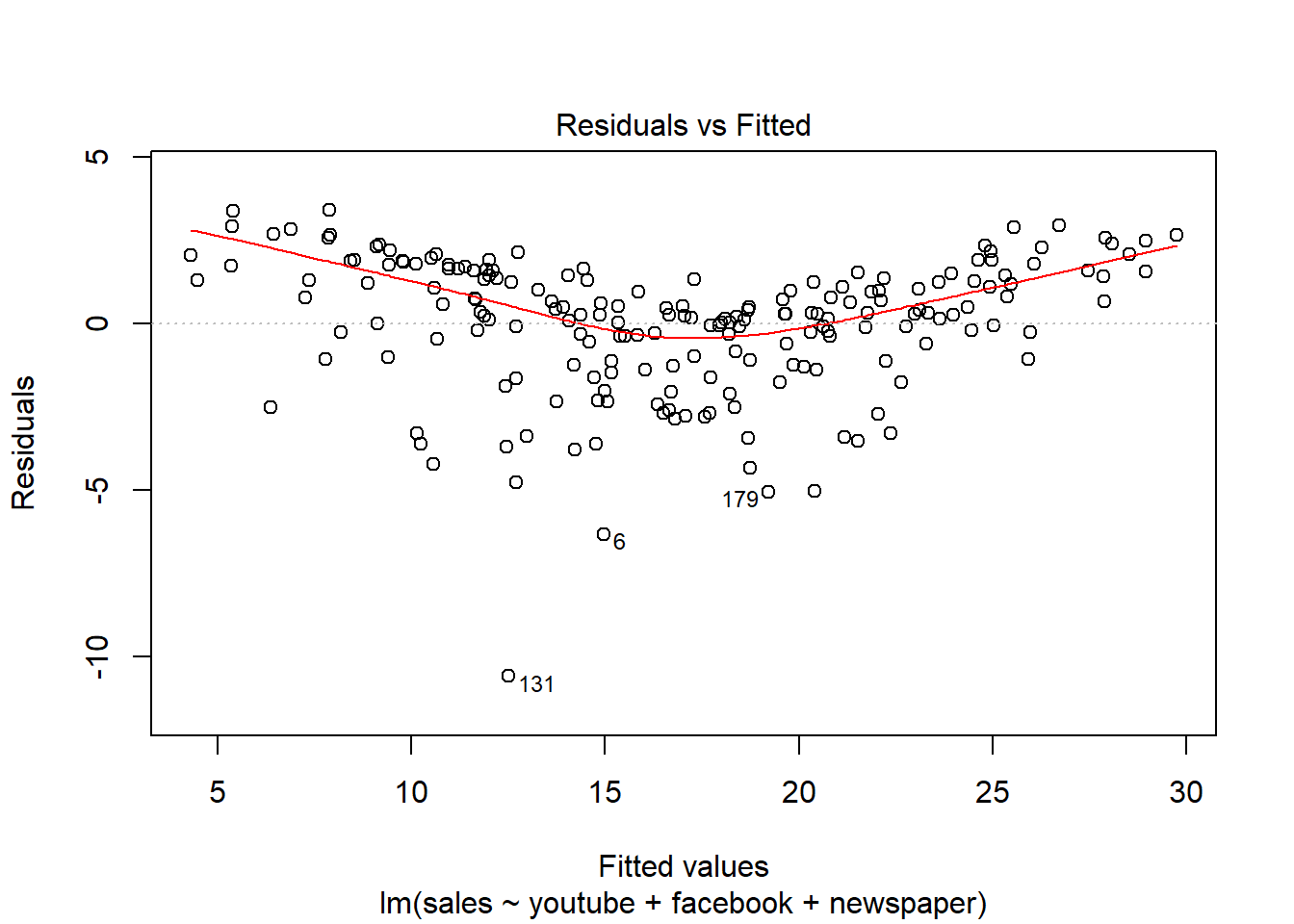
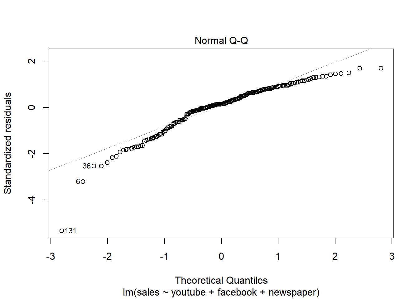
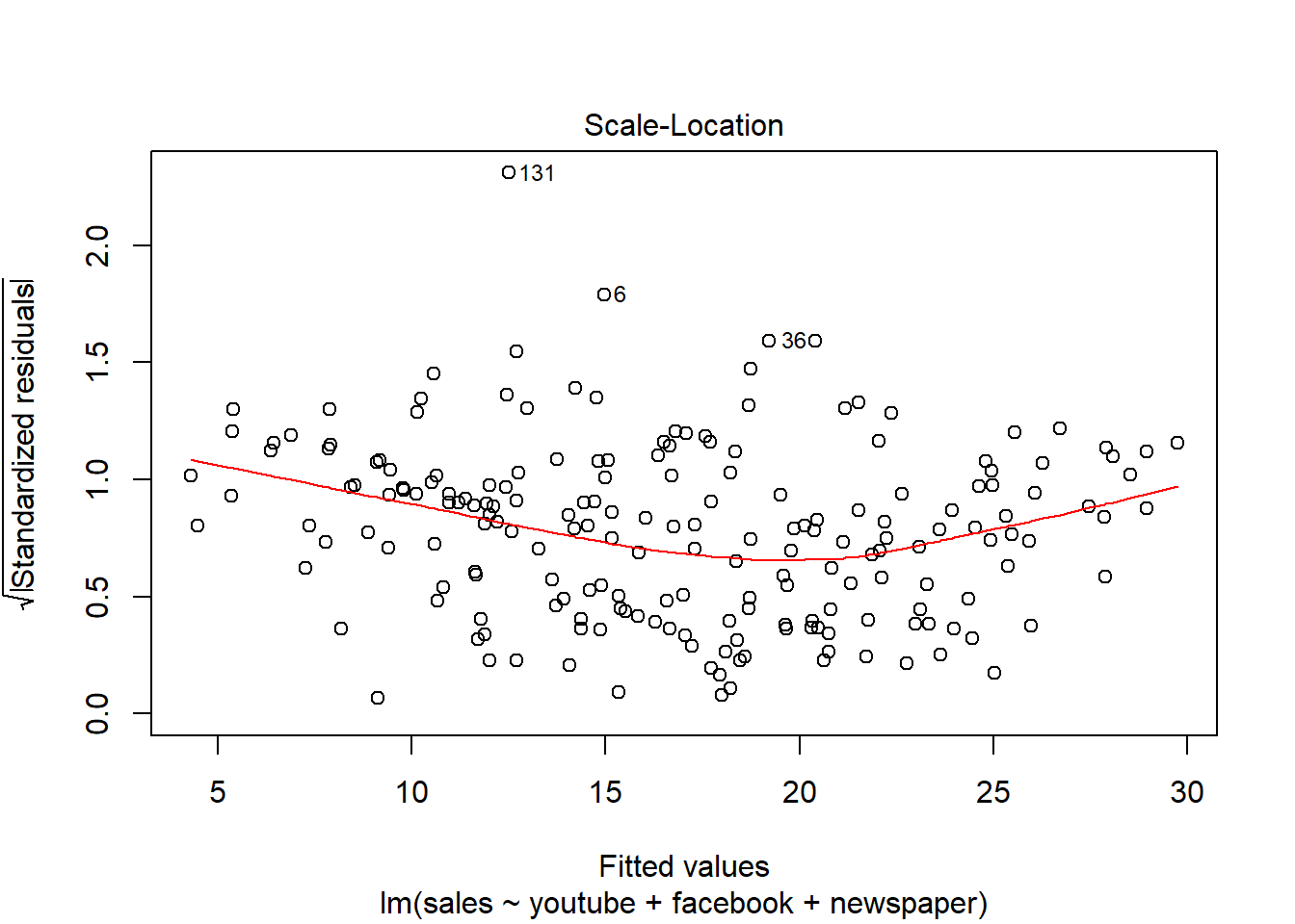
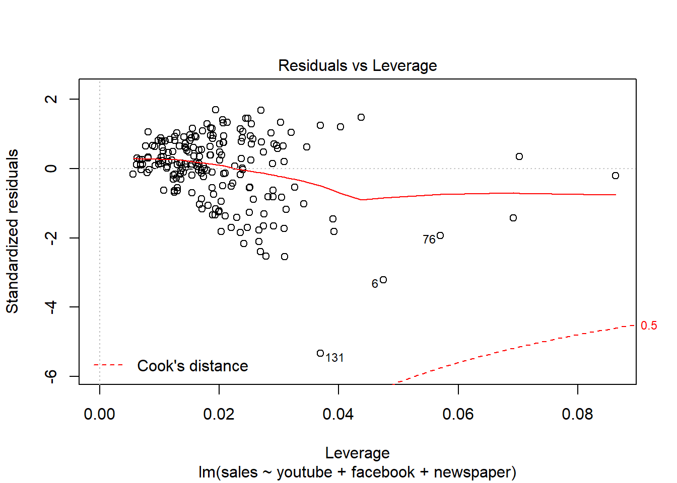
##
## Call:
## lm(formula = sales ~ youtube + facebook + newspaper, data = marketing)
##
## Residuals:
## Min 1Q Median 3Q Max
## -10.5932 -1.0690 0.2902 1.4272 3.3951
##
## Coefficients:
## Estimate Std. Error t value Pr(>|t|)
## (Intercept) 3.526667 0.374290 9.422 <2e-16 ***
## youtube 0.045765 0.001395 32.809 <2e-16 ***
## facebook 0.188530 0.008611 21.893 <2e-16 ***
## newspaper -0.001037 0.005871 -0.177 0.86
## ---
## Signif. codes: 0 '***' 0.001 '**' 0.01 '*' 0.05 '.' 0.1 ' ' 1
##
## Residual standard error: 2.023 on 196 degrees of freedom
## Multiple R-squared: 0.8972, Adjusted R-squared: 0.8956
## F-statistic: 570.3 on 3 and 196 DF, p-value: < 2.2e-16Modelo polinomial
- Hay una parabola sales - youtube
##
## Call:
## lm(formula = sales ~ youtube + I(youtube^2))
##
## Coefficients:
## (Intercept) youtube I(youtube^2)
## 7.337e+00 6.727e-02 -5.706e-05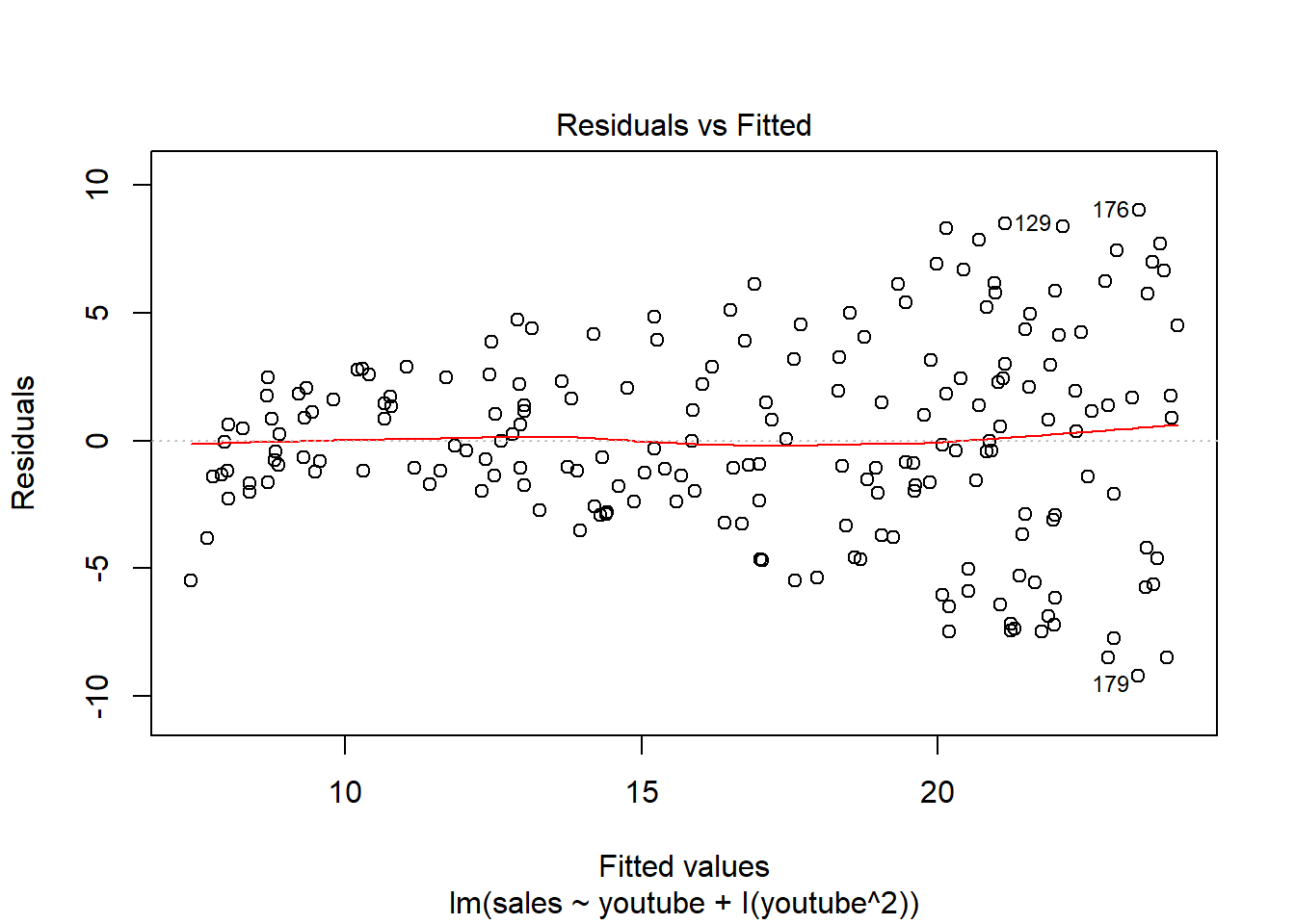
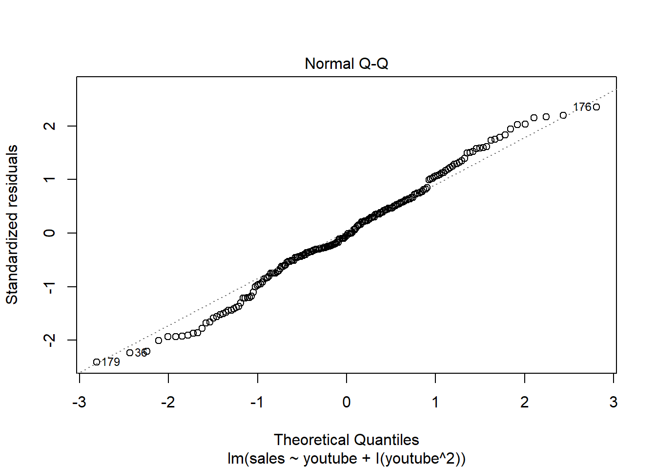
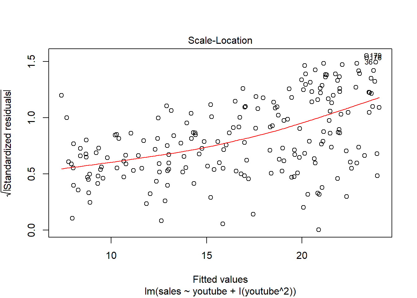
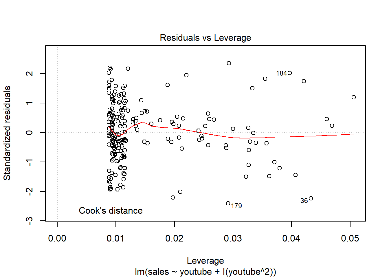
##
## Call:
## lm(formula = sales ~ youtube + I(youtube^2))
##
## Residuals:
## Min 1Q Median 3Q Max
## -9.2213 -2.1412 -0.1874 2.4106 9.0117
##
## Coefficients:
## Estimate Std. Error t value Pr(>|t|)
## (Intercept) 7.337e+00 7.911e-01 9.275 < 2e-16 ***
## youtube 6.727e-02 1.059e-02 6.349 1.46e-09 ***
## I(youtube^2) -5.706e-05 2.965e-05 -1.924 0.0557 .
## ---
## Signif. codes: 0 '***' 0.001 '**' 0.01 '*' 0.05 '.' 0.1 ' ' 1
##
## Residual standard error: 3.884 on 197 degrees of freedom
## Multiple R-squared: 0.619, Adjusted R-squared: 0.6152
## F-statistic: 160.1 on 2 and 197 DF, p-value: < 2.2e-164.3.3 Ejercicios del campus
Regresión - Ajustes: Fuel Efficiency of Automobiles
Usaremos el dataset FuelEfficiency.csv del CV. El objetivo es ajustar la eficiencia de consumo de gasoil (fuel). Los principales atributos son: GPM (gallons per 100 miles), MPG (miles per gallon), WT (weigth), DIS (distance), HP (horsepower), NC (number of cylinders).
- Importar el dataset y gráficamente encontrar relaciones entre las variables.
## Registered S3 method overwritten by 'GGally':
## method from
## +.gg ggplot2##
## Attaching package: 'GGally'## The following object is masked from 'package:dplyr':
##
## nasa## Parsed with column specification:
## cols(
## MPG = col_double(),
## GPM = col_double(),
## WT = col_double(),
## DIS = col_double(),
## NC = col_double(),
## HP = col_double(),
## ACC = col_double(),
## ET = col_double()
## )# Vamos a eliminar los atributos innecesarios como son ACC y ET
FuelEfficiency <- FuelEfficiency %>% select(-ACC, -ET)
head(FuelEfficiency)## # A tibble: 6 x 6
## MPG GPM WT DIS NC HP
## <dbl> <dbl> <dbl> <dbl> <dbl> <dbl>
## 1 16.9 5.92 4.36 350 8 155
## 2 15.5 6.45 4.05 351 8 142
## 3 19.2 5.21 3.60 267 8 125
## 4 18.5 5.40 3.94 360 8 150
## 5 30 3.33 2.15 98 4 68
## 6 27.5 3.64 2.56 134 4 95## MPG GPM WT DIS
## Min. :15.50 Min. :2.681 Min. :1.915 Min. : 85.0
## 1st Qu.:18.52 1st Qu.:3.292 1st Qu.:2.208 1st Qu.:105.0
## Median :24.25 Median :4.160 Median :2.685 Median :148.5
## Mean :24.76 Mean :4.331 Mean :2.863 Mean :177.3
## 3rd Qu.:30.38 3rd Qu.:5.398 3rd Qu.:3.410 3rd Qu.:229.5
## Max. :37.30 Max. :6.452 Max. :4.360 Max. :360.0
## NC HP
## Min. :4.000 Min. : 65.0
## 1st Qu.:4.000 1st Qu.: 78.5
## Median :4.500 Median :100.0
## Mean :5.395 Mean :101.7
## 3rd Qu.:6.000 3rd Qu.:123.8
## Max. :8.000 Max. :155.0# Realizando un plot, podemos encontrar relaciones interesantes entre las variables
plot(FuelEfficiency)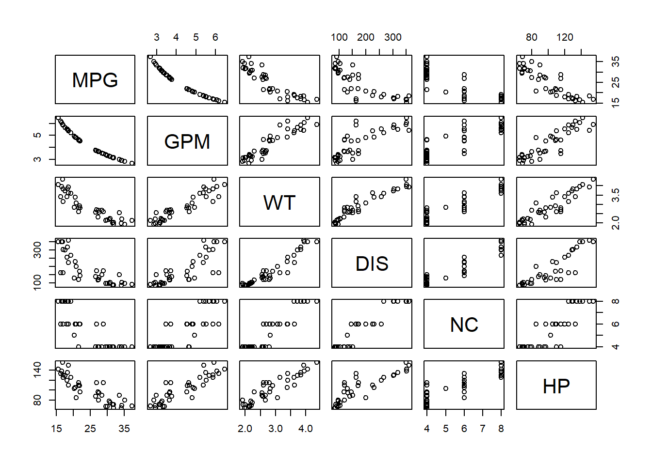
Analizando la representacion gráfica de las variables, podriamos observar relaciones directamente proporcionales como puede ser x=gpm y=wt, es decir, a mayor peso, mayor consumo, y tambien hay graficas inversamente proporcionales como puede ser x=hp y=mpg, es decir, a mayor potencia en caballos, recorre menos millas por galon (Que viene a ser lo mismo que indicar que mayor potencia, mayor consumo). Y tambien podemos observar algunas que quizas se ajusten mejor con funciones cuadraticas como puede ser x=mpg y=dis.
- Intentar un modelo de regresión lineal entre GPM y el resto de variables. Evaluar el modelo. ¿Con qué variables hay mayor relación?. Hacer gráficos de dataset junto con los modelos.
Vamos a intentar realizar un modelo de regresion lineal entre GPM y el resto de variables
## `geom_smooth()` using method = 'loess' and formula 'y ~ x'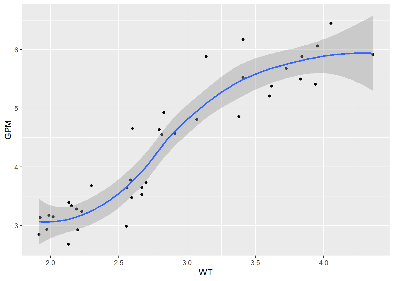
##
## Call:
## lm(formula = GPM ~ WT, data = FuelEfficiency)
##
## Coefficients:
## (Intercept) WT
## -0.006101 1.514798##
## Call:
## lm(formula = GPM ~ WT, data = FuelEfficiency)
##
## Residuals:
## Min 1Q Median 3Q Max
## -0.88072 -0.29041 0.00659 0.19021 1.13164
##
## Coefficients:
## Estimate Std. Error t value Pr(>|t|)
## (Intercept) -0.006101 0.302681 -0.02 0.984
## WT 1.514798 0.102721 14.75 <2e-16 ***
## ---
## Signif. codes: 0 '***' 0.001 '**' 0.01 '*' 0.05 '.' 0.1 ' ' 1
##
## Residual standard error: 0.4417 on 36 degrees of freedom
## Multiple R-squared: 0.858, Adjusted R-squared: 0.854
## F-statistic: 217.5 on 1 and 36 DF, p-value: < 2.2e-16- La informacion de los residuos nos indica la calidad del ajuste realizado, como se ajusta nuestro modelo a los datos del dataset
- Analizando el resumen de f1, podemos ver que el valor de R2 es 0.858, siendo un ajuste bastante cercano a 1, por lo que podriamos concluir que es un buen ajuste. 85.8% de la variabilidad de GPM viene reflejada por la variable WT.
- Observamos 36 grados de libertad posibles para estimar la variabilidad de los parametros y fiabilidad del ajuste.
- F-stadistico = 217.5 –> Alejado de 1 indica buen ajuste
- p-value: < 2.2e-16 –> Al ser un valor tan bajo rechazamos H0 aceptando H1, es decir, que si hay modelo.
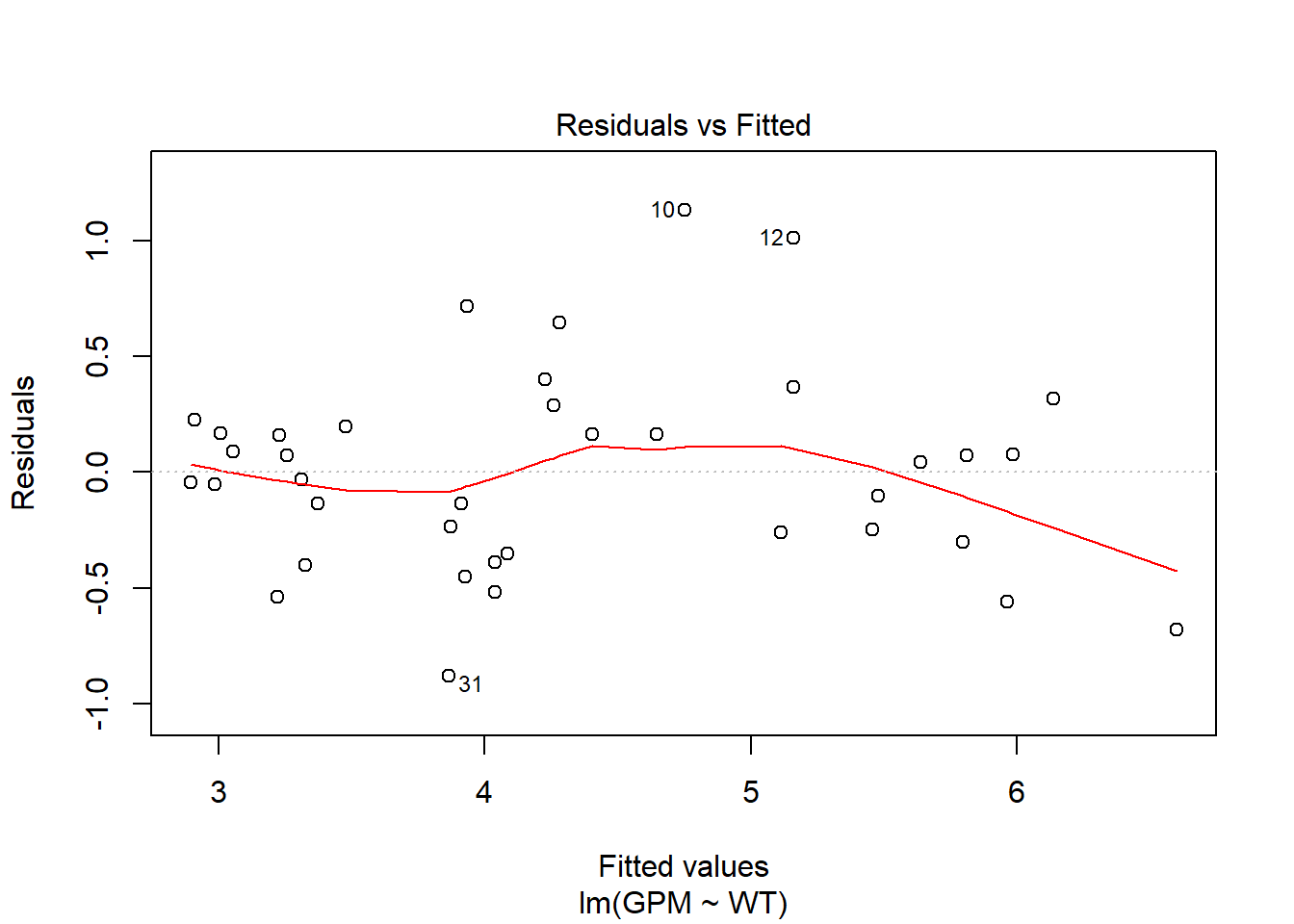

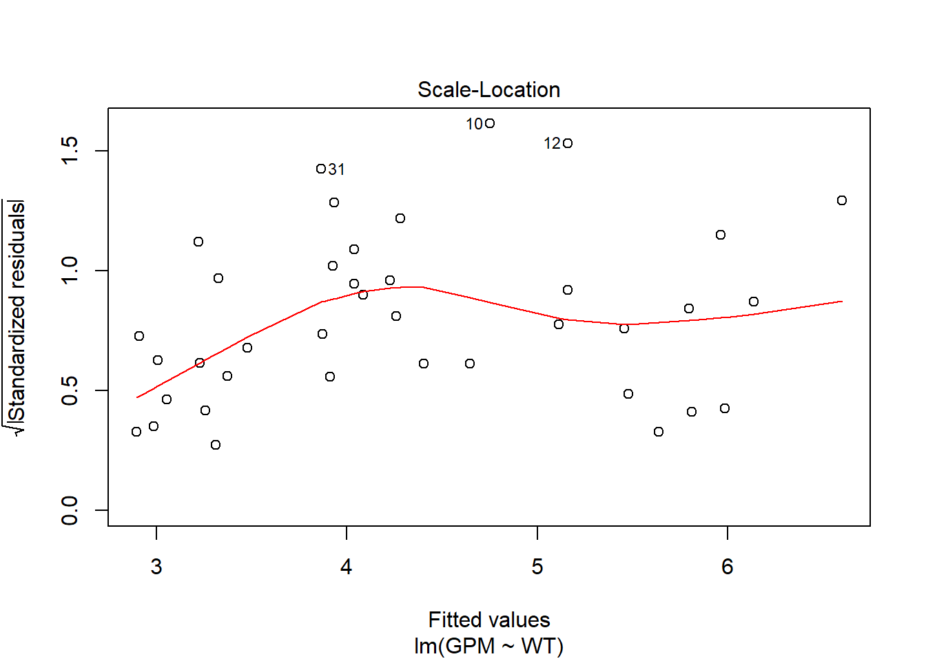
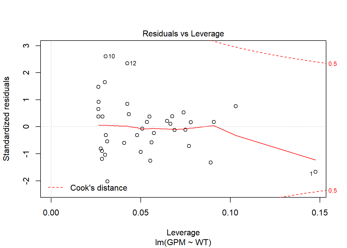 Analizamos las 4 graficas generadas por el plot:
- 1.- Residuos linealmente distribuidos, cerca del y = 0.
- 2.- Residuos están practicamente distribuidos siguiendo una normal, la y = x. Tambien me detecta outliers, valores importantes usando la distancia de Cook.
- 3.- Residuos están distribuidos aleatoriamente - mucha dispersión de los errores.
- 4.- Vemos los calculos de la distancia de Cook
## `geom_smooth()` using method = 'loess' and formula 'y ~ x'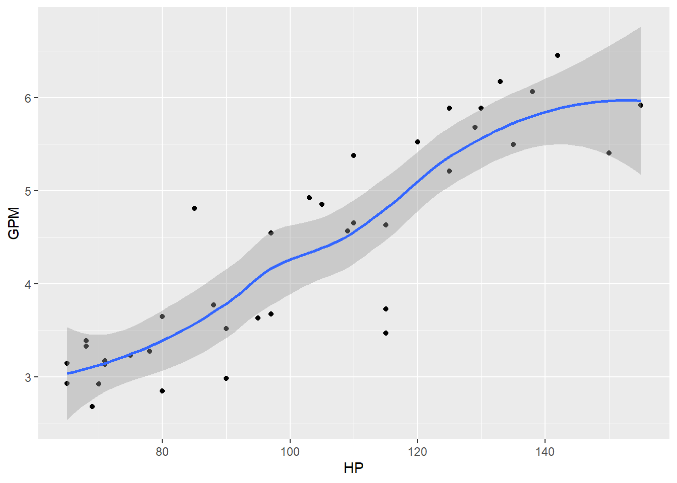
##
## Call:
## lm(formula = GPM ~ HP, data = FuelEfficiency)
##
## Coefficients:
## (Intercept) HP
## 0.3828 0.0388##
## Call:
## lm(formula = GPM ~ HP, data = FuelEfficiency)
##
## Residuals:
## Min 1Q Median 3Q Max
## -1.37328 -0.31944 -0.00157 0.38971 1.12686
##
## Coefficients:
## Estimate Std. Error t value Pr(>|t|)
## (Intercept) 0.382761 0.352319 1.086 0.285
## HP 0.038804 0.003354 11.568 1.1e-13 ***
## ---
## Signif. codes: 0 '***' 0.001 '**' 0.01 '*' 0.05 '.' 0.1 ' ' 1
##
## Residual standard error: 0.5396 on 36 degrees of freedom
## Multiple R-squared: 0.788, Adjusted R-squared: 0.7821
## F-statistic: 133.8 on 1 and 36 DF, p-value: 1.105e-13- La informacion de los residuos nos indica la calidad del ajuste realizado, como se ajusta nuestro modelo a los datos del dataset
- Analizando el resumen de f2, podemos ver que el valor de R2 es 0.788, siendo un ajuste bastante cercano a 1, es decir, siendo un ajuste aceptable. 78.8% de la variabilidad de GPM viene reflejada por la variable HP.
- Observamos 36 grados de libertad posibles para estimar la variabilidad de los parametros y fiabilidad del ajuste.
- F-stadistico = 133.8 –> Alejado de 1 indica buen ajuste
- p-value: = 1.105e-13 –> Al ser un valor tan bajo rechazamos H0 aceptando H1, es decir, que si hay modelo.
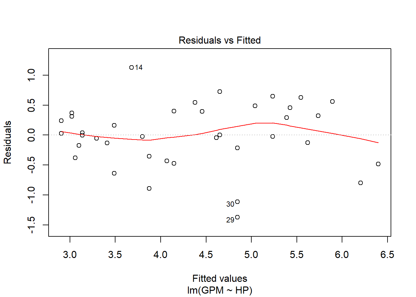
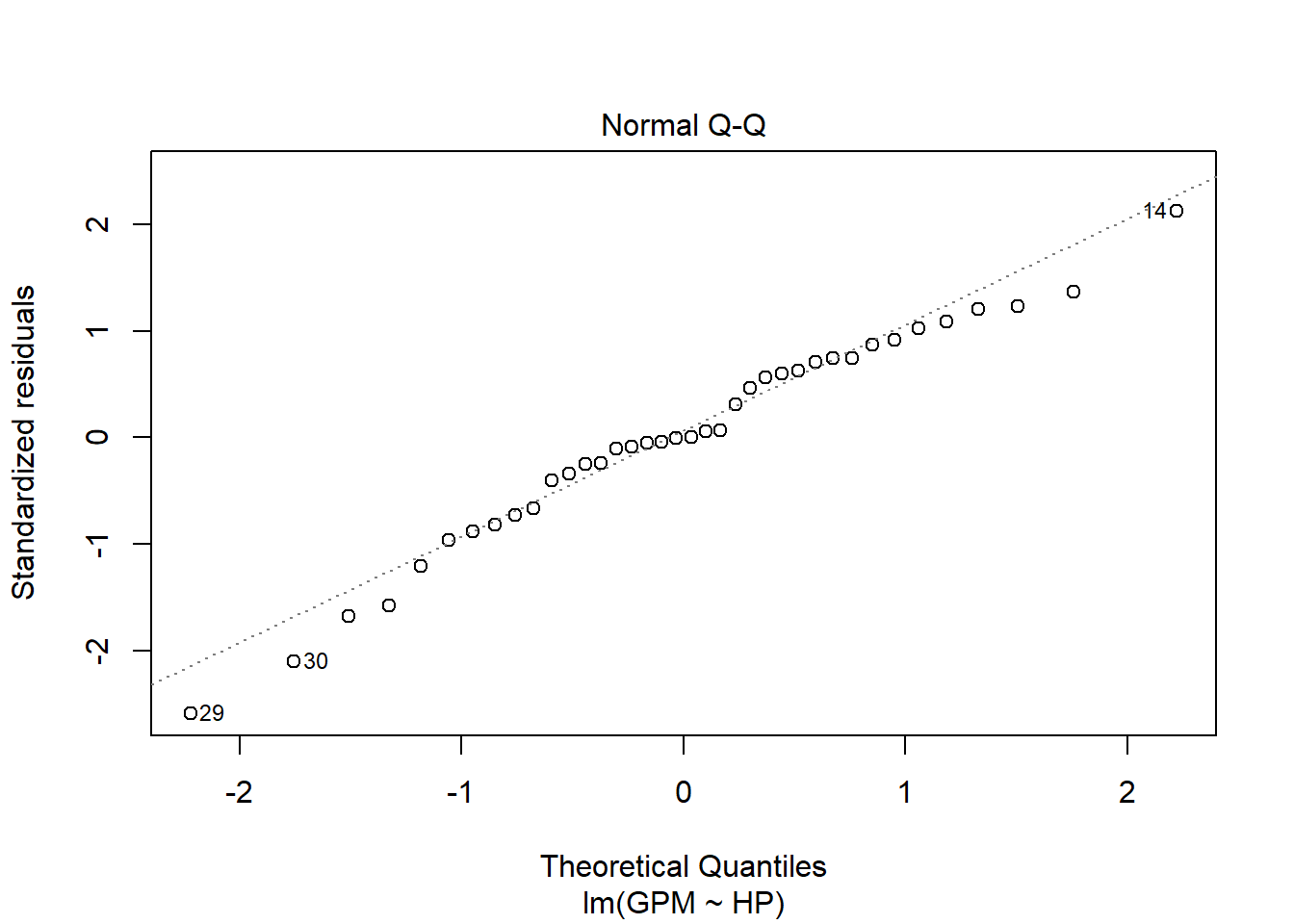
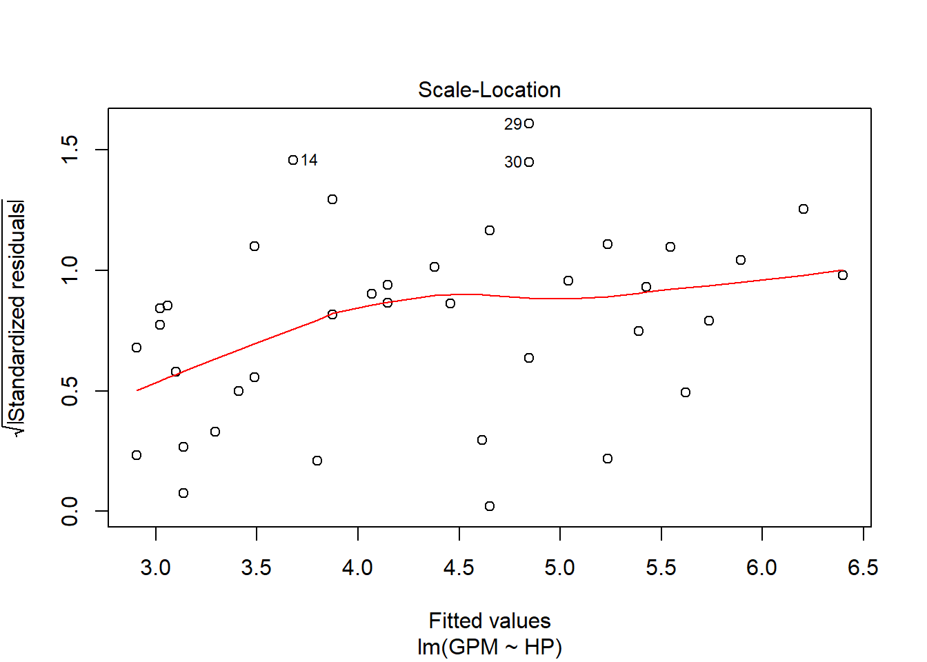
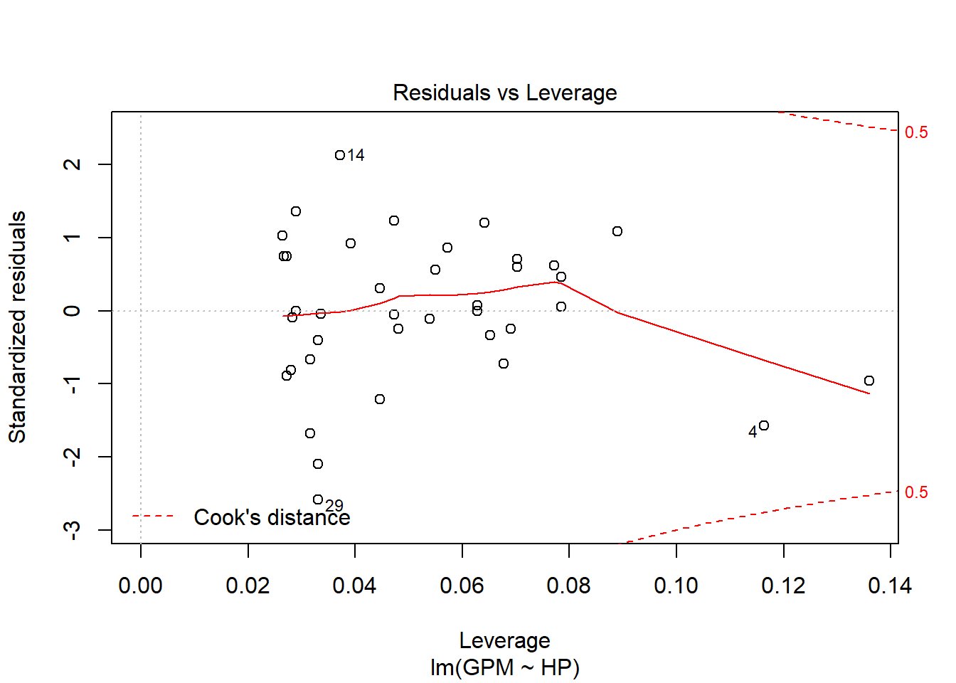
Analizamos las 4 graficas generadas por el plot
- 1.- Residuos linealmente distribuidos, cerca del y = 0.
- 2.- Residuos están practicamente distribuidos siguiendo una normal, la y = x. Tambien me detecta outliers, valores importantes usando la distancia de Cook.
- 3.- Residuos están distribuidos aleatoriamente - mucha dispersión de los errores.
- 4.- Vemos los calculos de la distancia de Cook
Para concluir este apartado, realizando una analisis superficial del resto de graficas posibles, es decir GPM~DIS y GPM~NC, la primera sería una grafica similar a las analizadas, las cuales presentan un modelo aceptable realizando una regresion lineal. La grafica GPM~NC sin embargo, no es adecuada para un ajuste lineal, pues su represetnacion gráfica no sigue ningun patron identificable
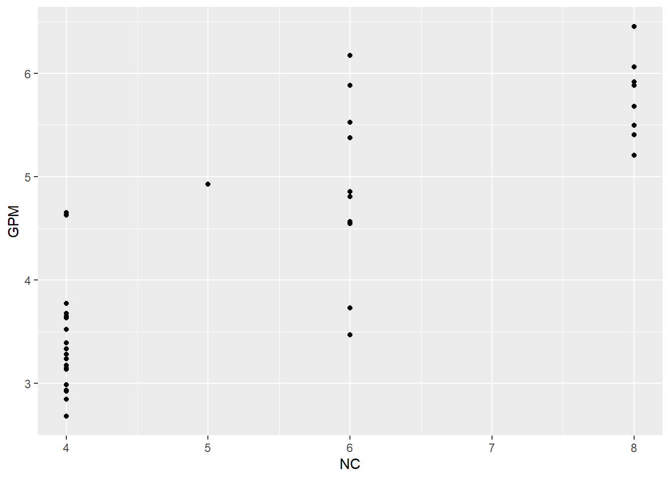
Realizando un analisis muy superficial, podemos ver que el consumo GPM no esta tan relacionado con la variable NC, al contrario que con otras variables. Sin embargo, es cierto, que hay una tendencia a tener un mayor consumo al poseer mas cilindros, pero el numero de cilindros no es del todo determinante del consumo del vehiculo, es decir, que entran en juego otros factores que propician que el consumo sea mayor.
- Intentar modelos de regresión de GPM con varias variables o incluso usando modelos no lineales. Evaluar los modelos. Hacer gráficos de dataset junto con los modelos.
Intentaremos analizar modelos de regresion multivariables, por ejemplo con todas las variables o con algunas en concreto (como puede ser cilindros + peso, para ver el efecto de los cilindros en el consumo de un coche)
##
## Call:
## lm(formula = GPM ~ ., data = FuelEfficiency)
##
## Coefficients:
## (Intercept) MPG WT DIS NC HP
## 6.219794 -0.131807 0.397032 -0.001392 0.070298 0.001035# Obtenemos la siguiente expresion
# GPM = 6.219794 - 0.131807*MPG + 0.397032*WT - 0.001392*DIS + 0.070298*NC + 0.001035*HP
summary(f3)##
## Call:
## lm(formula = GPM ~ ., data = FuelEfficiency)
##
## Residuals:
## Min 1Q Median 3Q Max
## -0.32836 -0.15706 -0.01305 0.12006 0.44487
##
## Coefficients:
## Estimate Std. Error t value Pr(>|t|)
## (Intercept) 6.219794 0.962248 6.464 2.85e-07 ***
## MPG -0.131807 0.015531 -8.487 1.07e-09 ***
## WT 0.397032 0.273554 1.451 0.156
## DIS -0.001392 0.001826 -0.762 0.451
## NC 0.070298 0.066613 1.055 0.299
## HP 0.001035 0.003420 0.303 0.764
## ---
## Signif. codes: 0 '***' 0.001 '**' 0.01 '*' 0.05 '.' 0.1 ' ' 1
##
## Residual standard error: 0.2079 on 32 degrees of freedom
## Multiple R-squared: 0.972, Adjusted R-squared: 0.9676
## F-statistic: 222.3 on 5 and 32 DF, p-value: < 2.2e-16Realizando el summary de f3, obtenemos la siguiente informacion:
- R2 = 0.972 y R2 ajustado = 0.9676, por lo que el modelo es casi perfecto y adicionalmente, no presenta sobrecarga, es decir, el valor de R2 ajustado no difiere casi con respecto a R2.
- Observamos 32 grados de libertad posibles para estimar la variabilidad de los parametros y fiabilidad del ajuste.
- F-stadistico = 222.3 –> Alejado de 1 indica buen ajuste
- p-value: < 2.2e-16 –> Al ser un valor tan bajo rechazamos H0 aceptando H1, es decir, que si hay modelo.
- Sin embargo, tambien podemos observar que hay variables despreciables, casi todas menos MPG, esto se debe a que al realizar un ajuste de GPM con MPG, al estar ambas relacionadas fuertemente, el resto de variables son despreciables. Esto es obvio ya que MPG indica las millas que podemos recorrer por galon de combustible y GPM expresa los galones que consumimos por cada milla de recorrido. Para poder observar un comportamiento algo diferente, optaremos por analizar GPM con respecto a todas las variables menos a MPG
##
## Call:
## lm(formula = GPM ~ WT + DIS + NC + HP, data = FuelEfficiency)
##
## Coefficients:
## (Intercept) WT DIS NC HP
## -1.620785 2.046783 -0.010236 0.187667 0.008787##
## Call:
## lm(formula = GPM ~ WT + DIS + NC + HP, data = FuelEfficiency)
##
## Residuals:
## Min 1Q Median 3Q Max
## -0.66694 -0.20075 0.01016 0.23997 0.62668
##
## Coefficients:
## Estimate Std. Error t value Pr(>|t|)
## (Intercept) -1.620785 0.477872 -3.392 0.001818 **
## WT 2.046783 0.341733 5.989 9.95e-07 ***
## DIS -0.010236 0.002662 -3.845 0.000522 ***
## NC 0.187667 0.115695 1.622 0.114301
## HP 0.008787 0.005852 1.502 0.142716
## ---
## Signif. codes: 0 '***' 0.001 '**' 0.01 '*' 0.05 '.' 0.1 ' ' 1
##
## Residual standard error: 0.3692 on 33 degrees of freedom
## Multiple R-squared: 0.909, Adjusted R-squared: 0.898
## F-statistic: 82.43 on 4 and 33 DF, p-value: < 2.2e-16Realizando el summary de f4, obtenemos la siguiente informacion:
- R2 = 0.909 y R2 ajustado = 0.898, por lo que el modelo es bueno y adicionalmente, no presenta sobrecarga, es decir, el valor de R2 ajustado no difiere casi con respecto a R2.
- Observamos 33 grados de libertad posibles para estimar la variabilidad de los parametros y fiabilidad del ajuste.
- F-stadistico = 82.43 –> Alejado de 1 indica buen ajuste
- p-value: < 2.2e-16 –> Al ser un valor tan bajo rechazamos H0 aceptando H1, es decir, que si hay modelo.
- Tambien se pueden despreciar las variables NC y HP pues no aportan mucha informacion o no suponen una perdida grande de informacion respecto a GPM, sin embargo, tanto el peso como la distancia afectan en gran parte a GPM.
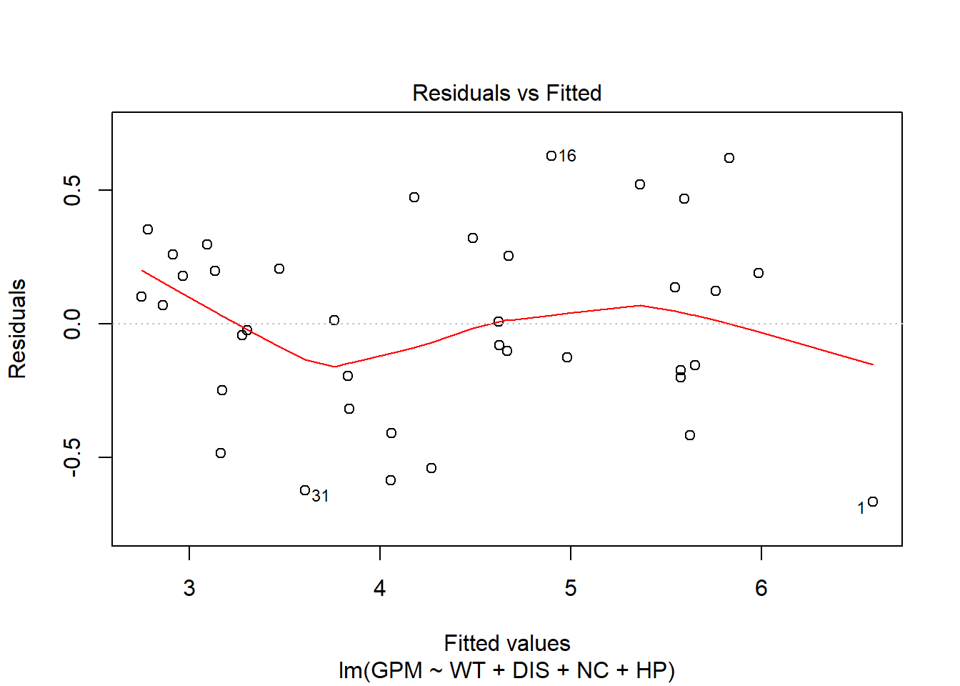
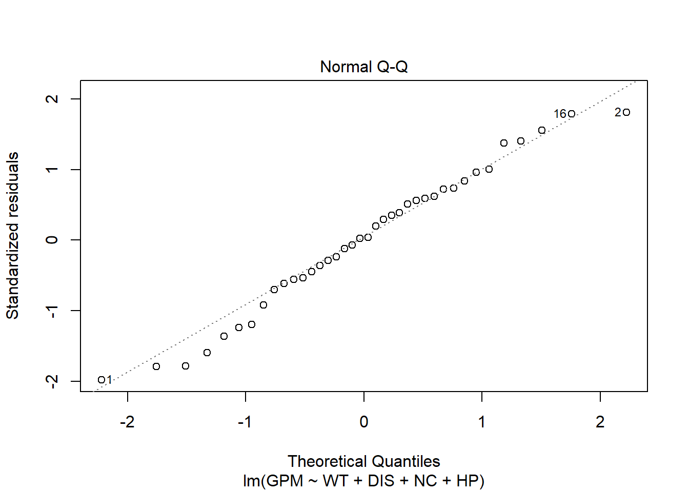
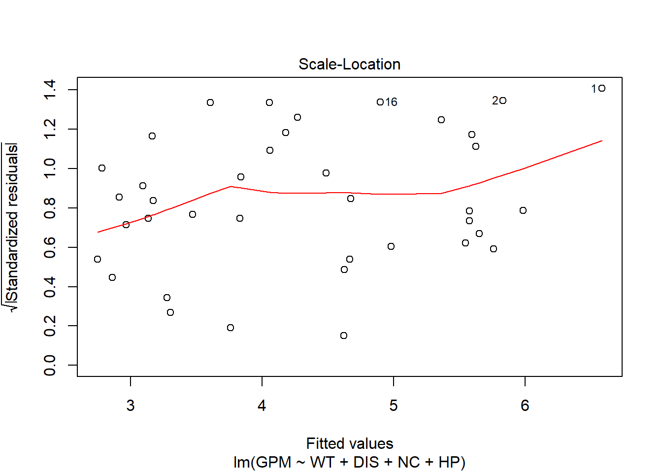
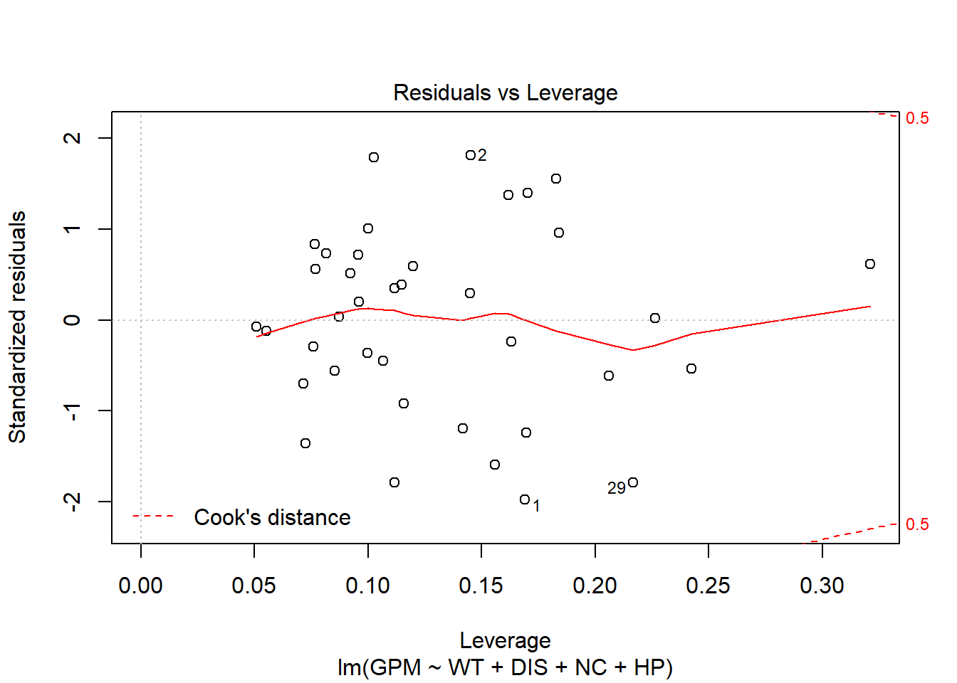
4.4 Text mining
4.4.1 Text Analytics con tenicas de clase
Librerias necesarias
library(devtools)
library(base64enc)
# si tienes problemas con la instalación normal instala twitteR de:
# install_github("geoffjentry/twitteR")
library(twitteR)
library(tm)
library(ggplot2)
library(ggmap)
library(httr)
library(wordcloud)
library (SnowballC)
library(RColorBrewer)
library(stringr)
library(lubridate)
library(data.table)
library(plyr)
library(wordcloud2)
library(rtweet)- Introduce tus claves en el documento para conectar con Twitter. Usa en el chunk la opción echo=FALSE, para no mostrar tus claves en el documento de salida.
## authenticate via web browser
token <- create_token(
app = "LabCompTwitter",
consumer_key = CONSUMER_KEY,
consumer_secret = CONSUMER_SECRET,
access_token = access_token,
access_secret = access_secret)## <Token>
## <oauth_endpoint>
## request: https://api.twitter.com/oauth/request_token
## authorize: https://api.twitter.com/oauth/authenticate
## access: https://api.twitter.com/oauth/access_token
## <oauth_app> LabCompTwitter
## key: 86f9HWLd89oXbwrbo2TbsxK1C
## secret: <hidden>
## <credentials> oauth_token, oauth_token_secret
## ---## [1] "Using direct authentication"Los siguientes apartados tiene eval = FALSE pues los tweets estan almacenados en un csv que obtuve anteriormente.
- Extraer de Twitter los tweets referentes a un tema que a ti te interese.
- Pasa los tweets a un dataframe y visualiza la cabeza del data frame.
- Graba los tweets en un csv.
PREPROCESAMIENTO DEL CSV
tweets2 <- read.csv("BunkerBoy.csv")
# Convierto a data frame el csv haciendo uso de la funcion glmpse de dplyr
bunkerBoy <- dplyr::glimpse(tweets2)## Rows: 5,000
## Columns: 17
## $ X <int> 1, 2, 3, 4, 5, 6, 7, 8, 9, 10, 11, 12, 13, 14, 15, 16...
## $ text <fct> "RT @AngelaBelcamino: Bunker bitch ass Trump.\n#Bunke...
## $ favorited <lgl> FALSE, FALSE, FALSE, FALSE, FALSE, FALSE, FALSE, FALS...
## $ favoriteCount <int> 0, 0, 0, 0, 0, 0, 0, 0, 0, 0, 0, 0, 0, 0, 0, 0, 0, 0,...
## $ replyToSN <fct> NA, NA, NA, NA, NA, NA, sanaayesha___, morethanmySLE,...
## $ created <fct> 2020-06-01 10:10:45, 2020-06-01 10:10:45, 2020-06-01 ...
## $ truncated <lgl> FALSE, FALSE, FALSE, FALSE, FALSE, FALSE, TRUE, TRUE,...
## $ replyToSID <dbl> NA, NA, NA, NA, NA, NA, 1.267390e+18, 1.267260e+18, N...
## $ id <dbl> 1.267398e+18, 1.267398e+18, 1.267398e+18, 1.267398e+1...
## $ replyToUID <dbl> NA, NA, NA, NA, NA, NA, 1.261510e+18, 8.123619e+17, N...
## $ statusSource <fct> <a href="http://twitter.com/download/iphone" rel="nof...
## $ screenName <fct> LouisGladney, luckystars14, gegesupreme, REALMrPoopy,...
## $ retweetCount <int> 540, 1097, 94, 5903, 5008, 559, 0, 0, 1758, 5903, 439...
## $ isRetweet <lgl> TRUE, TRUE, TRUE, TRUE, TRUE, TRUE, FALSE, FALSE, TRU...
## $ retweeted <lgl> FALSE, FALSE, FALSE, FALSE, FALSE, FALSE, FALSE, FALS...
## $ longitude <lgl> NA, NA, NA, NA, NA, NA, NA, NA, NA, NA, NA, NA, NA, N...
## $ latitude <lgl> NA, NA, NA, NA, NA, NA, NA, NA, NA, NA, NA, NA, NA, N...# perform a quick cleanup/transformation
# tweets.df = twListToDF(tweets2) - Esta no es necesaria pues los tweets ya estan en formato df
bunkerBoy$text <- sapply(bunkerBoy$text,function(x) iconv(x,to='UTF-8'))
bunkerBoy$created <- ymd_hms(bunkerBoy$created)
# comprobamos en que columnas hay valores NA
sapply(bunkerBoy, function(x) sum(is.na(x)))## X text favorited favoriteCount replyToSN
## 0 0 0 0 4816
## created truncated replyToSID id replyToUID
## 0 0 4834 0 4816
## statusSource screenName retweetCount isRetweet retweeted
## 0 0 0 0 0
## longitude latitude
## 5000 5000- ¿Cuantos tweets hay?
## [1] 5000- Analiza la estructura de la información que te has traido de Twitter.
## 'data.frame': 5000 obs. of 17 variables:
## $ X : int 1 2 3 4 5 6 7 8 9 10 ...
## $ text : chr "RT @AngelaBelcamino: Bunker bitch ass Trump.\n#BunkerBoy" "RT @Annmarie257257: Hide all you want we know what you are, coward. #BunkerBoy https://t.co/7J7jd1aisj" "RT @THENIGGAMATEO: Knocking on Trumps bunker door like #BunkerBoy #FuckTrumo https://t.co/MblAAkkIH2" "RT @acnewsitics: Trump turning off the lights at The White House describes the current situation in America per"| __truncated__ ...
## $ favorited : logi FALSE FALSE FALSE FALSE FALSE FALSE ...
## $ favoriteCount: int 0 0 0 0 0 0 0 0 0 0 ...
## $ replyToSN : Factor w/ 95 levels "1920ReporterGuy",..: NA NA NA NA NA NA 74 55 NA NA ...
## $ created : POSIXct, format: "2020-06-01 10:10:45" "2020-06-01 10:10:45" ...
## $ truncated : logi FALSE FALSE FALSE FALSE FALSE FALSE ...
## $ replyToSID : num NA NA NA NA NA ...
## $ id : num 1.27e+18 1.27e+18 1.27e+18 1.27e+18 1.27e+18 ...
## $ replyToUID : num NA NA NA NA NA ...
## $ statusSource : Factor w/ 23 levels "<a href=\"http://itunes.apple.com/us/app/twitter/id409789998?mt=12\" rel=\"nofollow\">Twitter for Mac</a>",..: 9 9 9 18 9 9 18 9 7 9 ...
## $ screenName : Factor w/ 3366 levels "___rifa","__drekaaaa__",..: 1872 1886 1118 2529 1696 2199 3087 2591 2777 2747 ...
## $ retweetCount : int 540 1097 94 5903 5008 559 0 0 1758 5903 ...
## $ isRetweet : logi TRUE TRUE TRUE TRUE TRUE TRUE ...
## $ retweeted : logi FALSE FALSE FALSE FALSE FALSE FALSE ...
## $ longitude : logi NA NA NA NA NA NA ...
## $ latitude : logi NA NA NA NA NA NA ...- ¿Cuantos usuarios distintos han participado?
## [1] 4997- ¿Cuantos tweets son re-tweets? (isRetweet)
## [1] 4437- ¿Cuantos tweets han sido re-tweeteados? (retweeted)
## [1] 0- ¿Cuál es el número medio de retweets? (retweetCount)
## [1] 1599.572- Da una lista con los distintos idiomas que se han usado al twitear este hashtag. (language)
Este apartado no se puede realizar porque el dataframe no obtiene ya la columna correspondiente al idioma. De todas formas, a la hora de extraer los tweets, especifique que fueran solo tweets en ingles, ya que los tweets extraidos estan relacionados mayormente con los acontencimientos en EEUU.
- Encontrar los nombres de usuarios de las 10 personas que más han participado. ¿Quién es el usuario que más ha participado?
## Emilinehope BoultThunder keithwhitson megthenoob73 LisaRogers1979
## 47 33 33 30 27
## imnotlewdmom mhshobeiri459 YulSun_K dawso_ Jz46977031
## 19 19 17 16 16## Emilinehope
## 47- Extraer en un data frame aquellos tweets re-tuiteados más de 5 veces (retweetCount).
# Primero eliminare los que son rt, para evitar la aparicion multiple de un mismo tweet
indices <- which(!bunkerBoy$isRetweet)
bunkerBoySinRt <- bunkerBoy[indices,]
# Selecciono aquellos que tengan rt count mayor a 5
topRt <- bunkerBoySinRt %>%
dplyr::filter(retweetCount >= 5)
head(rmarkdown::paged_table(topRt))## [1] 10 17- Aplicarle a los tweets las técnicas de Text-Mining vistas en clase:
- Haz pre-procesamiento adecuado.
- Calcula la media de la frecuencia de aparición de los términos
- Encuentra los términos que ocurren más de la media y guárdalos en un data.frame: término y su frecuencia. Usa knitr::kable en el .Rmd siempre que quieras visualizar los data.frame.
- Ordena este data.frame por la frecuencia
- Haz un plot de los términos más frecuentes. Si salen muchos términos visualiza un número adecuado de palabras para que se pueda ver algo.
- Genera diversos wordclouds y graba en disco el wordcloud generado.
- Busca información de paquete wordcloud2. Genera algún gráfico con este paquete.
toSpace <- content_transformer(function(x, pattern) gsub(pattern, " ", x))
toString <- content_transformer(function(x, from, to) gsub(from, to, x))
# El texto se encuentra en:
# Eliminar los usuarios @xxx y los hasthag #yyy
#docs <- str_extract_all(bunkerBoy$text, "@\\w+")
bunkerBoy2 <- bunkerBoy
bunkerBoy2$text <- stringr::str_replace_all(bunkerBoy2$text, "@\\w+"," ")
bunkerBoy2$text <- stringr::str_replace_all(bunkerBoy2$text, "#\\S+"," ")## Remove Hashtags
bunkerBoy2$text <- stringr::str_replace_all(bunkerBoy2$text, "http\\S+\\s*"," ")## Remove URLs
bunkerBoy2$text <- stringr::str_replace_all(bunkerBoy2$text, "http[[:alnum:]]*"," ")## Remove URLs
bunkerBoy2$text <- stringr::str_replace_all(bunkerBoy2$text, "http[[\\b+RT]]"," ")## Remove URLs
bunkerBoy2$text <- stringr::str_replace_all(bunkerBoy2$text, "[[:cntrl:]]"," ")
bunkerBoy2$text <- stringr::str_replace_all(bunkerBoy2$text, "#BunkerBoy"," ")
# Remover caracteres ascii extended
bunkerBoy2$text <- stringr::str_replace_all(bunkerBoy2$text, "[^\\x00-\\x7F]"," ")
docsCorpus <- Corpus(VectorSource(bunkerBoy2$text))
docsCorpus <- tm_map(docsCorpus, function(x) iconv(enc2utf8(x), sub = "byte"))## Warning in tm_map.SimpleCorpus(docsCorpus, function(x) iconv(enc2utf8(x), :
## transformation drops documents## Warning in tm_map.SimpleCorpus(docsCorpus, content_transformer(tolower)):
## transformation drops documents## Warning in tm_map.SimpleCorpus(docsCorpus, removeNumbers): transformation drops
## documents## Warning in tm_map.SimpleCorpus(docsCorpus, removePunctuation): transformation
## drops documents## Warning in tm_map.SimpleCorpus(docsCorpus, stripWhitespace): transformation
## drops documents## Warning in tm_map.SimpleCorpus(docsCorpus, removeWords, stopwords("english")):
## transformation drops documents## Warning in tm_map.SimpleCorpus(docsCorpus, toSpace, "rt"): transformation drops
## documents## <<DocumentTermMatrix (documents: 5000, terms: 2057)>>
## Non-/sparse entries: 38508/10246492
## Sparsity : 100%
## Maximal term length: 15
## Weighting : term frequency (tf)## know lights house bunker white trump
## 535 656 776 989 1049 1885##
## able abo abou absolute absolutely
## 1 1 1 1 1
## acab acces account accountability accurate
## 1 1 1 1 1
## across act acting action actions
## 1 1 1 1 1## freq
## 1 2 3 4 5 6 7 8 9 10 11 12 13 14 15
## 925 292 184 95 57 42 32 32 14 21 15 9 15 20 7set.seed(142)
# Distintas paletas de colores
# brewer.pal(6, "Dark2")
# brewer.pal(9,"YlGnBu")
#wordcloud(names(freq), freq, min.freq=350, max.words=50, scale=c(5, .1), colors=brewer.pal(6, "Dark2"))
#set.seed(42)
wordcloud(names(freq), freq, min.freq=25, max.words = 60)
wordcloud(names(freq), freq, scale=c(3,0.5), max.words=60, random.order=FALSE,
rot.per=0.10, use.r.layout=TRUE, colors=brewer.pal(6, "Dark2")) 
wordcloud(names(freq), freq, scale=c(3,0.5), max.words=60, random.order=FALSE,
rot.per=0.10, use.r.layout=TRUE, colors=brewer.pal(9,"Accent")) ## Warning in brewer.pal(9, "Accent"): n too large, allowed maximum for palette Accent is 8
## Returning the palette you asked for with that many colors
wordcloud(names(freq), freq, scale=c(3,0.5), max.words=60, random.order=FALSE,
rot.per=0.10, use.r.layout=TRUE, colors=brewer.pal(12,"Paired")) 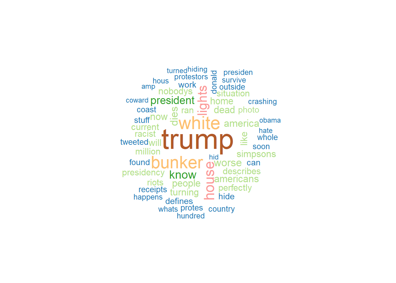
# Conversion a data frame de las frecuencias
freq.df <- as.data.frame(names(freq))
freq.df <- cbind(freq.df, freq)
names(freq.df) <- c("word", "freq")
wordcloud2(freq.df, color = "random-light", backgroundColor = "grey")- Para las 5 palabras más importantes de vuestro análisis encontrar palabras que estén relacionadas y guárdalas en un data.frame. Haz plot de las asociaciones.
## word freq
## 1 trump 1885
## 2 white 1049
## 3 bunker 989
## 4 house 776
## 5 lights 656
## 6 know 535top5 <- freq.ord$word[1:5]
top5 <- as.character(top5)
asociaciones <- findAssocs(dtm, top5[1], corlimit=0.35)
asociaciones## $trump
## white house
## 0.46 0.37# convertimos en un data.frame
lista.asoc <- lapply(asociaciones, function(x) data.frame(rhs = names(x), cor = x, stringsAsFactors = FALSE))
#crear un dataframe con tres columnas
df.asoc <- dplyr::bind_rows(lista.asoc, .id = "lhs")
ggplot(df.asoc, aes(y = df.asoc[, 2])) + geom_point(aes(x = df.asoc[, 3]),
data = df.asoc[,2:3], size = 3) +
ggtitle(paste(top5[1], "relacionado con...")) +
ylab("Palabras")+
xlab("correlación")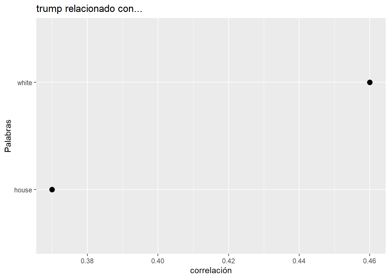
## $white
## house current describes perfectly situation nobodys turning home
## 0.85 0.49 0.49 0.49 0.49 0.48 0.48 0.47
## trump lights
## 0.46 0.45# convertimos en un data.frame
lista.asoc2 <- lapply(asociaciones2, function(x) data.frame(rhs = names(x), cor = x, stringsAsFactors = FALSE))
#crear un dataframe con tres columnas
df.asoc2 <- dplyr::bind_rows(lista.asoc2, .id = "lhs")
ggplot(df.asoc2, aes(y = df.asoc2[, 2])) + geom_point(aes(x = df.asoc2[, 3]),
data = df.asoc2[,2:3], size = 3) +
ggtitle(paste(top5[2], "relacionado con...")) +
ylab("Palabras")+
xlab("correlación")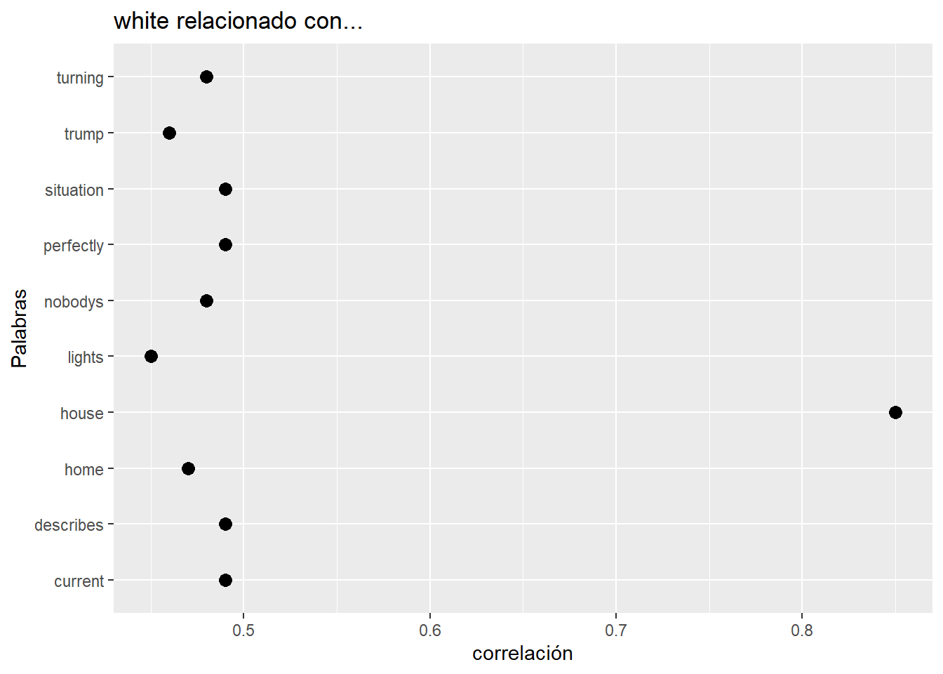
## $bunker
## crashing hous hundred outside protestors survive can
## 0.45 0.45 0.45 0.45 0.45 0.45 0.44# convertimos en un data.frame
lista.asoc3 <- lapply(asociaciones3, function(x) data.frame(rhs = names(x), cor = x, stringsAsFactors = FALSE))
#crear un dataframe con tres columnas
df.asoc3 <- dplyr::bind_rows(lista.asoc3, .id = "lhs")
ggplot(df.asoc3, aes(y = df.asoc3[, 2])) + geom_point(aes(x = df.asoc3[, 3]),
data = df.asoc3[,2:3], size = 3) +
ggtitle(paste(top5[3], "relacionado con...")) +
ylab("Palabras")+
xlab("correlación")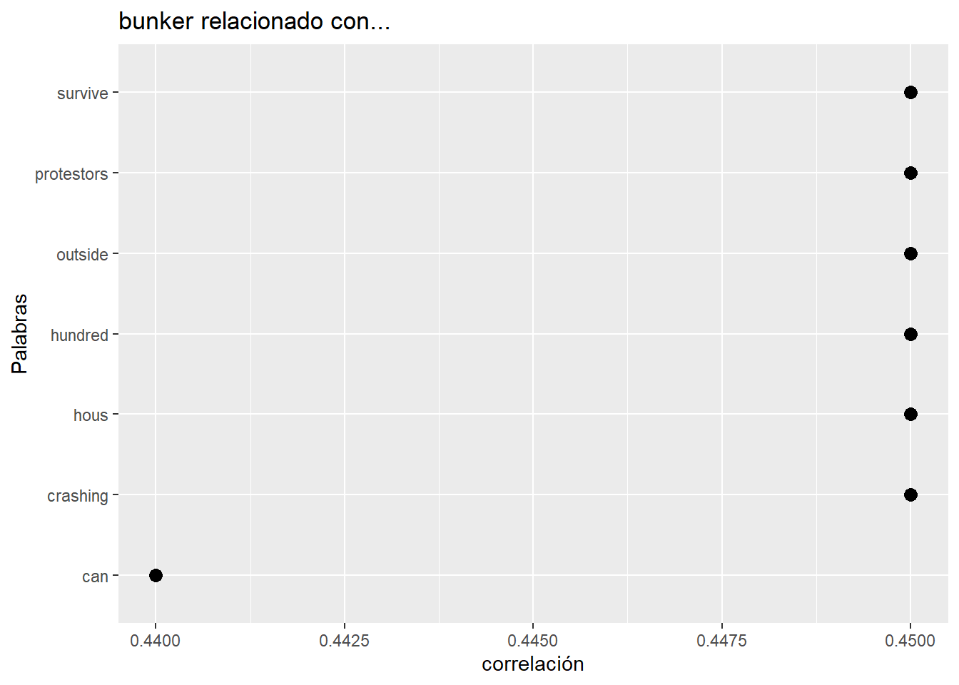
## $house
## white current describes perfectly situation turning nobodys home
## 0.85 0.58 0.58 0.58 0.58 0.57 0.56 0.55
## lights
## 0.55# convertimos en un data.frame
lista.asoc4 <- lapply(asociaciones4, function(x) data.frame(rhs = names(x), cor = x, stringsAsFactors = FALSE))
#crear un dataframe con tres columnas
df.asoc4 <- dplyr::bind_rows(lista.asoc4, .id = "lhs")
ggplot(df.asoc4, aes(y = df.asoc4[, 2])) + geom_point(aes(x = df.asoc4[, 3]),
data = df.asoc4[,2:3], size = 3) +
ggtitle(paste(top5[4], "relacionado con...")) +
ylab("Palabras")+
xlab("correlación")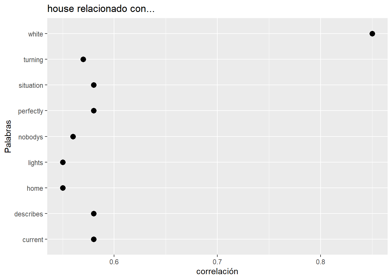
## $lights
## turning current describes perfectly situation
## 0.73 0.71 0.71 0.71 0.71# convertimos en un data.frame
lista.asoc5 <- lapply(asociaciones5, function(x) data.frame(rhs = names(x), cor = x, stringsAsFactors = FALSE))
#crear un dataframe con tres columnas
df.asoc5 <- dplyr::bind_rows(lista.asoc5, .id = "lhs")
ggplot(df.asoc5, aes(y = df.asoc5[, 2])) + geom_point(aes(x = df.asoc5[, 3]),
data = df.asoc5[,2:3], size = 3) +
ggtitle(paste(top5[5], "relacionado con...")) +
ylab("Palabras")+
xlab("correlación")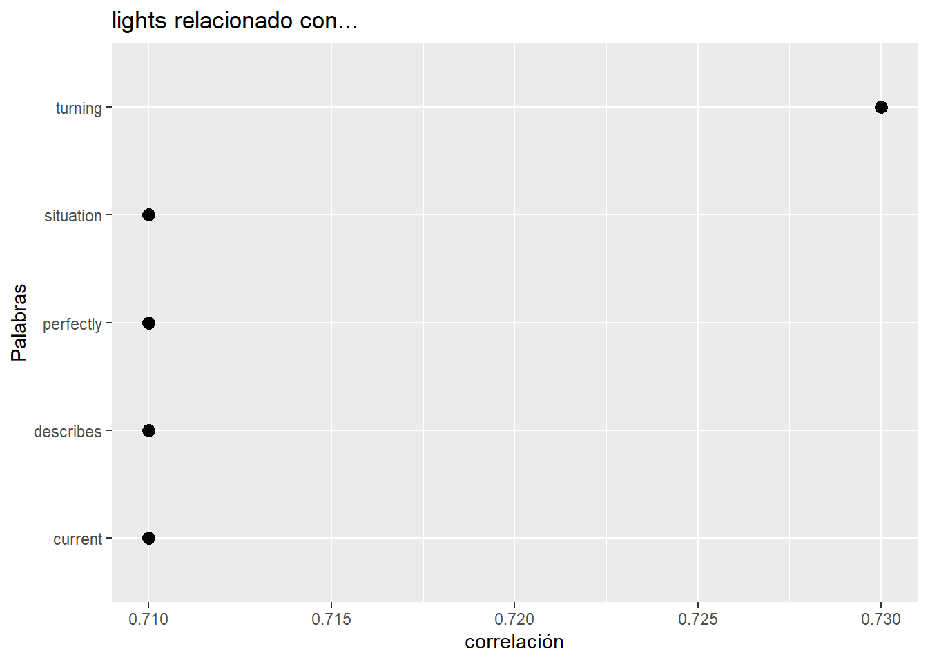
# Unimos los dataframes
df.asociaciones <- rbind(df.asoc, df.asoc2, df.asoc3, df.asoc4, df.asoc5)
df.asociaciones## lhs rhs cor
## 1 trump white 0.46
## 2 trump house 0.37
## 3 white house 0.85
## 4 white current 0.49
## 5 white describes 0.49
## 6 white perfectly 0.49
## 7 white situation 0.49
## 8 white nobodys 0.48
## 9 white turning 0.48
## 10 white home 0.47
## 11 white trump 0.46
## 12 white lights 0.45
## 13 bunker crashing 0.45
## 14 bunker hous 0.45
## 15 bunker hundred 0.45
## 16 bunker outside 0.45
## 17 bunker protestors 0.45
## 18 bunker survive 0.45
## 19 bunker can 0.44
## 20 house white 0.85
## 21 house current 0.58
## 22 house describes 0.58
## 23 house perfectly 0.58
## 24 house situation 0.58
## 25 house turning 0.57
## 26 house nobodys 0.56
## 27 house home 0.55
## 28 house lights 0.55
## 29 lights turning 0.73
## 30 lights current 0.71
## 31 lights describes 0.71
## 32 lights perfectly 0.71
## 33 lights situation 0.71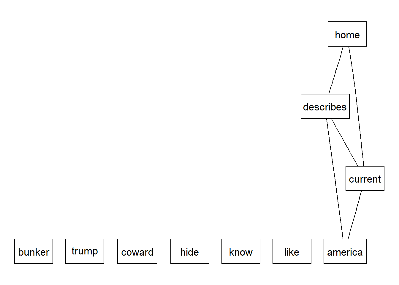
- Haz plot con los dispositivos desde los que se han mandado los tweets.
# plot por emisor
# encode tweet source as iPhone, iPad, Android or Web
encodeSource <- function(x) {
if(x=="<a href=\"http://twitter.com/download/iphone\" rel=\"nofollow\">Twitter for iPhone</a>"){
gsub("<a href=\"http://twitter.com/download/iphone\" rel=\"nofollow\">Twitter for iPhone</a>", "iphone", x,fixed=TRUE)
}else if(x=="<a href=\"http://twitter.com/#!/download/ipad\" rel=\"nofollow\">Twitter for iPad</a>"){
gsub("<a href=\"http://twitter.com/#!/download/ipad\" rel=\"nofollow\">Twitter for iPad</a>","ipad",x,fixed=TRUE)
}else if(x=="<a href=\"http://twitter.com/download/android\" rel=\"nofollow\">Twitter for Android</a>"){
gsub("<a href=\"http://twitter.com/download/android\" rel=\"nofollow\">Twitter for Android</a>","android",x,fixed=TRUE)
} else if(x=="<a href=\"http://twitter.com\" rel=\"nofollow\">Twitter Web Client</a>"){
gsub("<a href=\"http://twitter.com\" rel=\"nofollow\">Twitter Web Client</a>","Web",x,fixed=TRUE)
} else if(x=="<a href=\"http://www.twitter.com\" rel=\"nofollow\">Twitter for Windows Phone</a>"){
gsub("<a href=\"http://www.twitter.com\" rel=\"nofollow\">Twitter for Windows Phone</a>","windows phone",x,fixed=TRUE)
}else if(x=="<a href=\"http://dlvr.it\" rel=\"nofollow\">dlvr.it</a>"){
gsub("<a href=\"http://dlvr.it\" rel=\"nofollow\">dlvr.it</a>","dlvr.it",x,fixed=TRUE)
}else if(x=="<a href=\"http://ifttt.com\" rel=\"nofollow\">IFTTT</a>"){
gsub("<a href=\"http://ifttt.com\" rel=\"nofollow\">IFTTT</a>","ifttt",x,fixed=TRUE)
}else if(x=="<a href=\"http://earthquaketrack.com\" rel=\"nofollow\">EarthquakeTrack.com</a>"){
gsub("<a href=\"http://earthquaketrack.com\" rel=\"nofollow\">EarthquakeTrack.com</a>","earthquaketrack",x,fixed=TRUE)
}else if(x=="<a href=\"http://www.didyoufeel.it/\" rel=\"nofollow\">Did You Feel It</a>"){
gsub("<a href=\"http://www.didyoufeel.it/\" rel=\"nofollow\">Did You Feel It</a>","did_you_feel_it",x,fixed=TRUE)
}else if(x=="<a href=\"http://www.mobeezio.com/apps/earthquake\" rel=\"nofollow\">Earthquake Mobile</a>"){
gsub("<a href=\"http://www.mobeezio.com/apps/earthquake\" rel=\"nofollow\">Earthquake Mobile</a>","earthquake_mobile",x,fixed=TRUE)
}else if(x=="<a href=\"http://www.facebook.com/twitter\" rel=\"nofollow\">Facebook</a>"){
gsub("<a href=\"http://www.facebook.com/twitter\" rel=\"nofollow\">Facebook</a>","facebook",x,fixed=TRUE)
}else {
"others"
}
}bunkerBoy$tweetSource = sapply(bunkerBoy$statusSource, function(sourceSystem) encodeSource(sourceSystem))
ggplot(bunkerBoy[bunkerBoy$tweetSource != 'others',], aes(tweetSource)) + geom_bar(fill = "aquamarine4") +
theme(legend.position="none",
axis.title.x = element_blank(),
axis.text.x = element_text(angle = 45, hjust = 1)) +
ylab("Number of tweets") 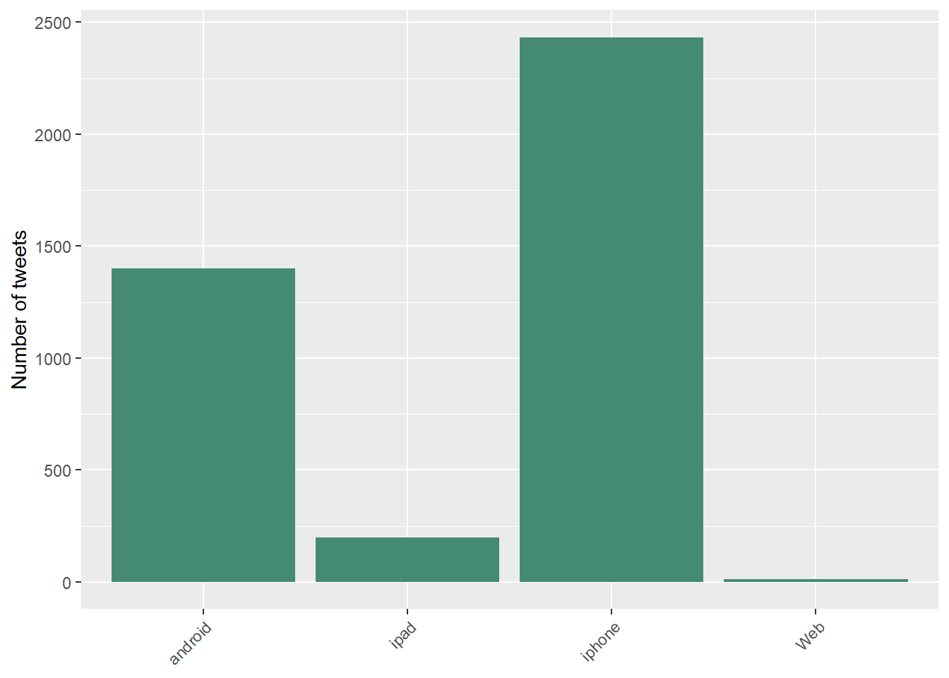
- Para la palabra más frecuente de tu análisis busca y graba en un data.frame en los tweets en los que está dicho término. El data.frame tendrá como columnas: término, usuario, texto.
# Selecciono el termino que mas aparece
mostFreq <- top5[1]
# Obtengo los indices donde aparece la palabra mas frecuente
# Hago uso del dataframe sin los rt para que no se repitan
indices <- which(grepl(mostFreq, bunkerBoySinRt$text))
# Creo un dataset con las columnas que me interesan
df <- bunkerBoySinRt %>%
dplyr::select(screenName, text) %>%
dplyr::mutate(termino = mostFreq)
df <- df[indices,]
# Ordeno las columnas
df <- df[, c(3,1,2)]Quito las librerias para que no haya problemas al compilar el book
4.4.2 Text Analytics con tidytext
Librerias necesarias
library(rtweet)
library(twitteR)
library(tm)
library(wordcloud)
library(wordcloud2)
library(RColorBrewer)
library(tidyverse)
library(tidytext)
library(igraph)
library(ggraph)
library(stringr)
library(ggplot2)
library(ggrepel)
library(lubridate)bunkerBoy <- read.csv("BunkerBoy.csv")
bunkerBoy$created <- ymd_hms(bunkerBoy$created)
bunkerBoy$text <- sapply(bunkerBoy$text,function(x) iconv(x,to='UTF-8'))
str(bunkerBoy)## 'data.frame': 5000 obs. of 17 variables:
## $ X : int 1 2 3 4 5 6 7 8 9 10 ...
## $ text : chr "RT @AngelaBelcamino: Bunker bitch ass Trump.\n#BunkerBoy" "RT @Annmarie257257: Hide all you want we know what you are, coward. #BunkerBoy https://t.co/7J7jd1aisj" "RT @THENIGGAMATEO: Knocking on Trumps bunker door like #BunkerBoy #FuckTrumo https://t.co/MblAAkkIH2" "RT @acnewsitics: Trump turning off the lights at The White House describes the current situation in America per"| __truncated__ ...
## $ favorited : logi FALSE FALSE FALSE FALSE FALSE FALSE ...
## $ favoriteCount: int 0 0 0 0 0 0 0 0 0 0 ...
## $ replyToSN : Factor w/ 95 levels "1920ReporterGuy",..: NA NA NA NA NA NA 74 55 NA NA ...
## $ created : POSIXct, format: "2020-06-01 10:10:45" "2020-06-01 10:10:45" ...
## $ truncated : logi FALSE FALSE FALSE FALSE FALSE FALSE ...
## $ replyToSID : num NA NA NA NA NA ...
## $ id : num 1.27e+18 1.27e+18 1.27e+18 1.27e+18 1.27e+18 ...
## $ replyToUID : num NA NA NA NA NA ...
## $ statusSource : Factor w/ 23 levels "<a href=\"http://itunes.apple.com/us/app/twitter/id409789998?mt=12\" rel=\"nofollow\">Twitter for Mac</a>",..: 9 9 9 18 9 9 18 9 7 9 ...
## $ screenName : Factor w/ 3366 levels "___rifa","__drekaaaa__",..: 1872 1886 1118 2529 1696 2199 3087 2591 2777 2747 ...
## $ retweetCount : int 540 1097 94 5903 5008 559 0 0 1758 5903 ...
## $ isRetweet : logi TRUE TRUE TRUE TRUE TRUE TRUE ...
## $ retweeted : logi FALSE FALSE FALSE FALSE FALSE FALSE ...
## $ longitude : logi NA NA NA NA NA NA ...
## $ latitude : logi NA NA NA NA NA NA ...## X
## 1 1
## 2 2
## 3 3
## 4 4
## 5 5
## 6 6
## text
## 1 RT @AngelaBelcamino: Bunker bitch ass Trump.\n#BunkerBoy
## 2 RT @Annmarie257257: Hide all you want we know what you are, coward. #BunkerBoy https://t.co/7J7jd1aisj
## 3 RT @THENIGGAMATEO: Knocking on Trumps bunker door like #BunkerBoy #FuckTrumo https://t.co/MblAAkkIH2
## 4 RT @acnewsitics: Trump turning off the lights at The White House describes the current situation in America perfectly. Nobody's home.\n\n#Bunâ\200¦
## 5 RT @4everNeverTrump: Trump ran to a bunker which can survive a 747 crashing into it because a few hundred protestors outside the White Housâ\200¦
## 6 RT @mjfree: So Biden is out on the streets talking to angry, grief-stricken Americans while #BunkerBoy Trump hides in a bunker?
## favorited favoriteCount replyToSN created truncated replyToSID
## 1 FALSE 0 <NA> 2020-06-01 10:10:45 FALSE NA
## 2 FALSE 0 <NA> 2020-06-01 10:10:45 FALSE NA
## 3 FALSE 0 <NA> 2020-06-01 10:10:44 FALSE NA
## 4 FALSE 0 <NA> 2020-06-01 10:10:43 FALSE NA
## 5 FALSE 0 <NA> 2020-06-01 10:10:43 FALSE NA
## 6 FALSE 0 <NA> 2020-06-01 10:10:42 FALSE NA
## id replyToUID
## 1 1.267398e+18 NA
## 2 1.267398e+18 NA
## 3 1.267398e+18 NA
## 4 1.267398e+18 NA
## 5 1.267398e+18 NA
## 6 1.267398e+18 NA
## statusSource
## 1 <a href="http://twitter.com/download/iphone" rel="nofollow">Twitter for iPhone</a>
## 2 <a href="http://twitter.com/download/iphone" rel="nofollow">Twitter for iPhone</a>
## 3 <a href="http://twitter.com/download/iphone" rel="nofollow">Twitter for iPhone</a>
## 4 <a href="https://mobile.twitter.com" rel="nofollow">Twitter Web App</a>
## 5 <a href="http://twitter.com/download/iphone" rel="nofollow">Twitter for iPhone</a>
## 6 <a href="http://twitter.com/download/iphone" rel="nofollow">Twitter for iPhone</a>
## screenName retweetCount isRetweet retweeted longitude latitude
## 1 LouisGladney 540 TRUE FALSE NA NA
## 2 luckystars14 1097 TRUE FALSE NA NA
## 3 gegesupreme 94 TRUE FALSE NA NA
## 4 REALMrPoopy 5903 TRUE FALSE NA NA
## 5 kojo_XO 5008 TRUE FALSE NA NA
## 6 natashainoz 559 TRUE FALSE NA NA## [1] 5000 17## [1] "RT @AngelaBelcamino: Bunker bitch ass Trump.\n#BunkerBoy"
## [2] "RT @Annmarie257257: Hide all you want we know what you are, coward. #BunkerBoy https://t.co/7J7jd1aisj"
## [3] "RT @THENIGGAMATEO: Knocking on Trumps bunker door like #BunkerBoy #FuckTrumo https://t.co/MblAAkkIH2"
## [4] "RT @acnewsitics: Trump turning off the lights at The White House describes the current situation in America perfectly. Nobody's home.\n\n#Bunâ\200¦"
## [5] "RT @4everNeverTrump: Trump ran to a bunker which can survive a 747 crashing into it because a few hundred protestors outside the White Housâ\200¦"
## [6] "RT @mjfree: So Biden is out on the streets talking to angry, grief-stricken Americans while #BunkerBoy Trump hides in a bunker?"Formato Tidy y Limpieza tweets
tweets_tidy <-
bunkerBoy %>%
mutate(text = str_replace_all(text, '(<a href=\"|http|https|" rel=\"nofollow\">|</a>)[^([:blank:]|\\"|<|&|#\n\r)]+', ""))## X favorited favoriteCount replyToSN created truncated
## 1 1 FALSE 0 <NA> 2020-06-01 10:10:45 FALSE
## 1.1 1 FALSE 0 <NA> 2020-06-01 10:10:45 FALSE
## 1.2 1 FALSE 0 <NA> 2020-06-01 10:10:45 FALSE
## 1.3 1 FALSE 0 <NA> 2020-06-01 10:10:45 FALSE
## 1.4 1 FALSE 0 <NA> 2020-06-01 10:10:45 FALSE
## 1.5 1 FALSE 0 <NA> 2020-06-01 10:10:45 FALSE
## replyToSID id replyToUID
## 1 NA 1.267398e+18 NA
## 1.1 NA 1.267398e+18 NA
## 1.2 NA 1.267398e+18 NA
## 1.3 NA 1.267398e+18 NA
## 1.4 NA 1.267398e+18 NA
## 1.5 NA 1.267398e+18 NA
## statusSource
## 1 <a href="http://twitter.com/download/iphone" rel="nofollow">Twitter for iPhone</a>
## 1.1 <a href="http://twitter.com/download/iphone" rel="nofollow">Twitter for iPhone</a>
## 1.2 <a href="http://twitter.com/download/iphone" rel="nofollow">Twitter for iPhone</a>
## 1.3 <a href="http://twitter.com/download/iphone" rel="nofollow">Twitter for iPhone</a>
## 1.4 <a href="http://twitter.com/download/iphone" rel="nofollow">Twitter for iPhone</a>
## 1.5 <a href="http://twitter.com/download/iphone" rel="nofollow">Twitter for iPhone</a>
## screenName retweetCount isRetweet retweeted longitude latitude
## 1 LouisGladney 540 TRUE FALSE NA NA
## 1.1 LouisGladney 540 TRUE FALSE NA NA
## 1.2 LouisGladney 540 TRUE FALSE NA NA
## 1.3 LouisGladney 540 TRUE FALSE NA NA
## 1.4 LouisGladney 540 TRUE FALSE NA NA
## 1.5 LouisGladney 540 TRUE FALSE NA NA
## word
## 1 rt
## 1.1 angelabelcamino
## 1.2 bunker
## 1.3 bitch
## 1.4 ass
## 1.5 trump## [1] "X" "favorited" "favoriteCount" "replyToSN"
## [5] "created" "truncated" "replyToSID" "id"
## [9] "replyToUID" "statusSource" "screenName" "retweetCount"
## [13] "isRetweet" "retweeted" "longitude" "latitude"
## [17] "word"## # A tibble: 12 x 2
## word lexicon
## <chr> <chr>
## 1 a SMART
## 2 a's SMART
## 3 able SMART
## 4 about SMART
## 5 above SMART
## 6 according SMART
## 7 you onix
## 8 young onix
## 9 younger onix
## 10 youngest onix
## 11 your onix
## 12 yours onix## [1] 90833mis_tokens <- mis_tokens %>%
anti_join(tibble(word = tm::stopwords("es")))%>%
anti_join(tibble(word = tm::stopwords("en")))%>%
anti_join(tibble(word = tm::stopwords("french")))## Joining, by = "word"
## Joining, by = "word"
## Joining, by = "word"## [1] 57489## [1] "rt" "angelabelcamino" "bunker" "bitch"
## [5] "ass" "trump"## # A tibble: 3,056 x 2
## word n
## <chr> <int>
## 1 rt 4440
## 2 bunkerboy 3005
## 3 trump 1872
## 4 white 1048
## 5 bunker 975
## 6 house 775
## 7 lights 651
## 8 ðÿ 643
## 9 know 535
## 10 realdonaldtrump 530
## # ... with 3,046 more rows## [1] "2020-06-01 09:42:49 UTC"## [1] "2020-06-01 10:10:45 UTC"## [1] 5000 17bunkerBoy %>%
ts_plot("seconds") +
ggplot2::theme_minimal() +
ggplot2::labs(
x = NULL, y = NULL,
title = "Frecuencia de tuits en el espacio temporal",
subtitle = "Minutos",
caption = "#BunkerBoy"
)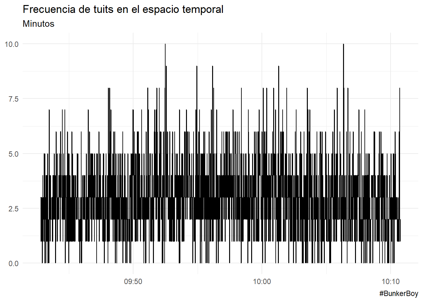
bunkerBoy %>%
ts_plot("minuts") +
ggplot2::theme_minimal() +
ggplot2::labs(
x = NULL, y = NULL,
title = "Frecuencia de tuits en el espacio temporal",
subtitle = "Minutos",
caption = "#BunkerBoy"
)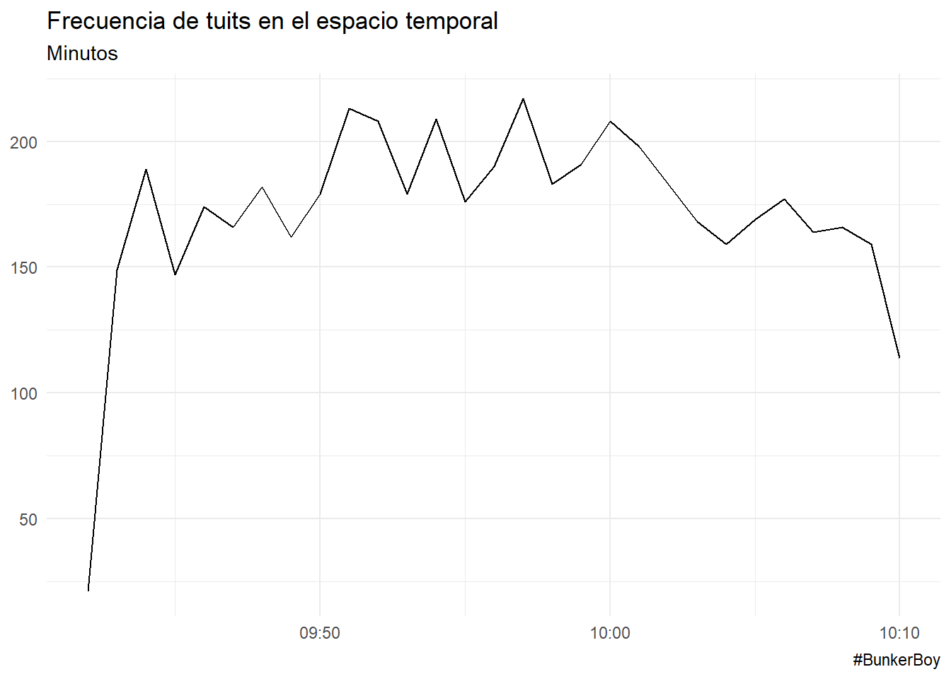
Preprocesamiento
mis_tokens <- mis_tokens %>%
filter(!str_detect(word, "[0-9]"),
word != "on",
word != "rt",
word != "t",
word != "realdonaldtrump",
!str_detect(word, "[^\\x00-\\x7F]"), #♣ Elimino los caracteres ascii extended
!str_detect(word, "[a-z]_"),
!str_detect(word, ":"))
# inspeccionar y volver a limpiar
head(mis_tokens$word,20) ## [1] "angelabelcamino" "bunker" "bitch" "ass"
## [5] "trump" "bunkerboy" "hide" "want"
## [9] "know" "coward" "bunkerboy" "theniggamateo"
## [13] "knocking" "trumps" "bunker" "door"
## [17] "like" "bunkerboy" "fucktrumo" "acnewsitics"Palabras más frecuentes - wordcloud
## Joining, by = "word"mis_tokens %>%
count(word, sort = TRUE) %>%
filter(n > 400) %>%
mutate(word = reorder(word, n)) %>%
ggplot(aes(word, n)) + geom_col(fill = "dodgerblue4") +
xlab(NULL) + coord_flip() + ggtitle("Palabras más comunes")
mis_tokens %>%
count(word, sort = TRUE) %>%
mutate(word = reorder(word, n)) %>%
dplyr::filter(n > 500 ) %>%
ggplot(aes(word, n)) +
ggplot2::labs(
y = "# veces que aparece",
x = "Palabra",
title = "Palabras más repetidas (> 500 veces)"
) +
geom_col() +
coord_flip() +
theme_minimal()
Construimos el wordcloud
mis_tokens %>%
count(word, sort = TRUE) %>%
dplyr::filter(n > 100 ) %>%
with(wordcloud::wordcloud(words = word,
freq = n,
max.words = 300,
random.order = FALSE,
rot.per = 0.25,colors=brewer.pal(6, "Dark2")))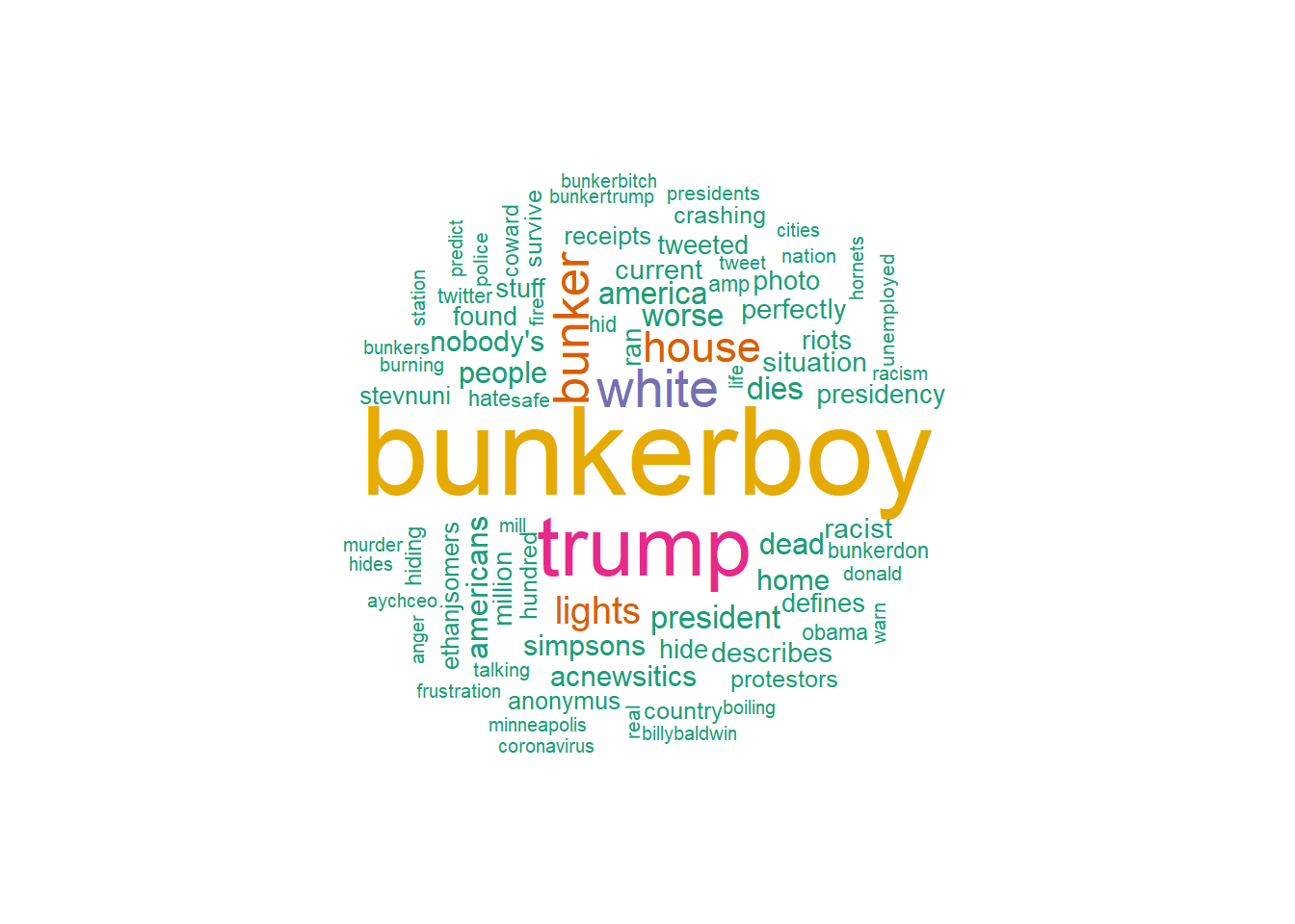
Analisis de sentimientos
La función inner_join() añade la información de sentimiento de esa palabra.
## Joining, by = "word"sentiment_mis_tokens_bing %>%
summarise(Negative = sum(sentiment == "negative"),
positive = sum(sentiment == "positive"))## Negative positive
## 1 4516 2805sentiment_mis_tokens_bing %>%
group_by(sentiment) %>%
count(word, sort = TRUE) %>%
filter(n > 50) %>%
ggplot(aes(word, n, fill = sentiment)) + geom_col(show.legend = FALSE) +
coord_flip() + facet_wrap(~sentiment, scales = "free_y") +
ggtitle("Contribución al sentimiento") + xlab(NULL) + ylab(NULL)+
theme()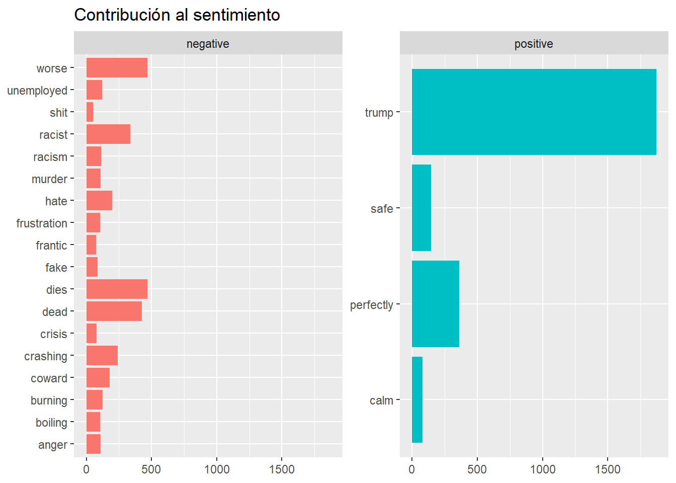
O en el mismo gráfico juntamos los sentimientos positivos y negativos:
sentiment_mis_tokens_bing %>%
group_by(sentiment) %>%
count(word, sort = TRUE) %>%
filter(n>50) %>%
mutate(n = ifelse(sentiment == "negative", -n, n)) %>%
ggplot(aes(word, n, fill = sentiment)) + geom_col() + coord_flip() +
ggtitle("Contribución al sentimiento") +
theme_minimal()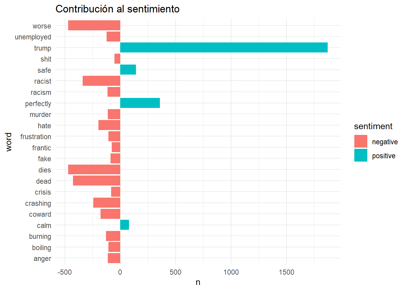
nrc proporciona la etiqueta (anger, anticipation, disgust, fear, joy, negative, positive, sadness, surprise or trust) a las palabras.
Analizamos cuantas palabras aparecen con cada uno de estos sentimientos:
sentiment_mis_tokens_nrc <-
mis_tokens %>%
inner_join(get_sentiments("nrc")) %>%
group_by(word, sentiment) %>%
count(word, sort = TRUE) %>%
filter(n > 150) %>%
ggplot(aes(x = n, y = word, fill = n)) +
geom_bar(stat = "identity", alpha = 0.8) +
facet_wrap(~ sentiment, ncol = 5) ## Joining, by = "word"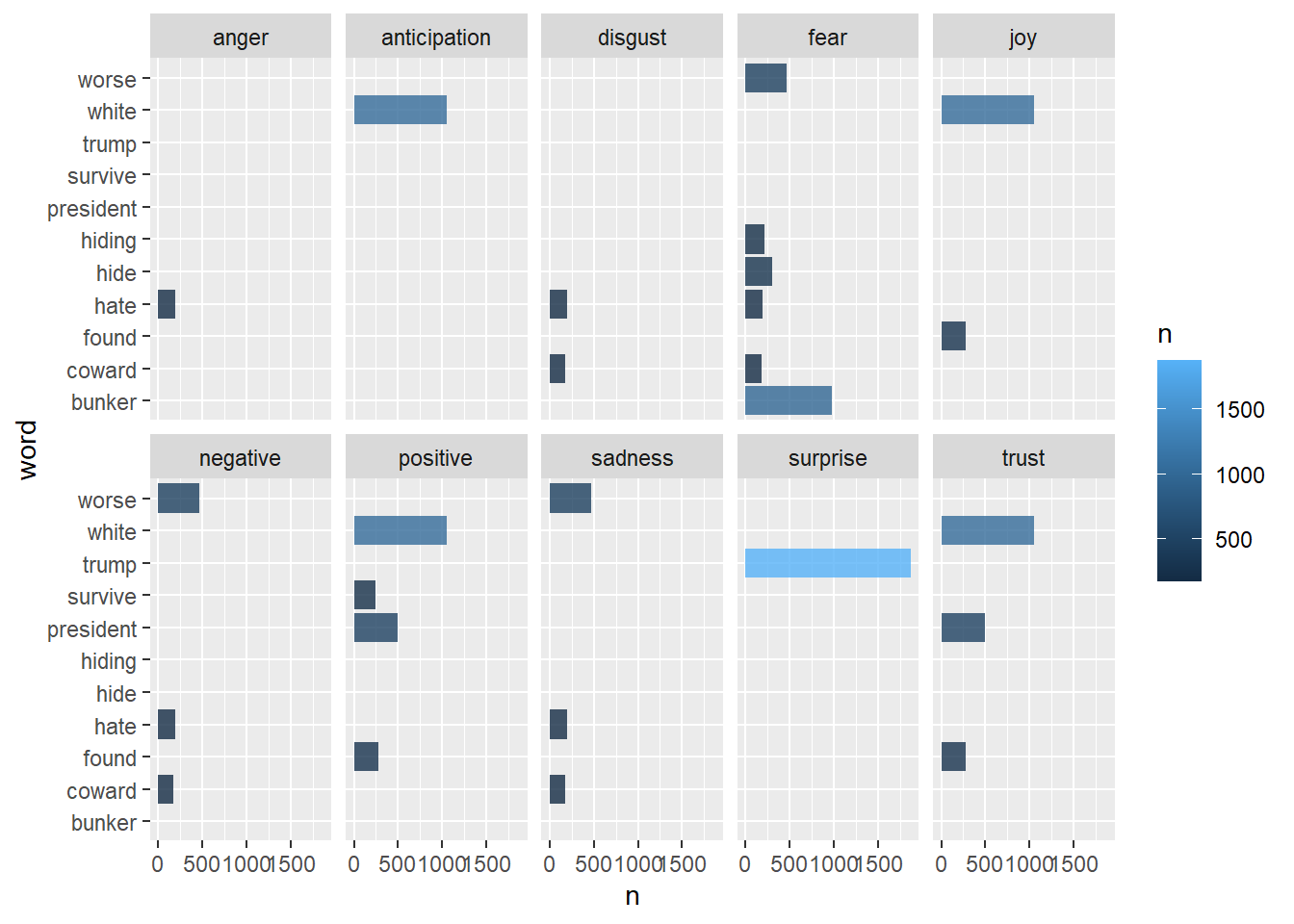
mis_tokens %>%
inner_join(get_sentiments("nrc")) %>%
group_by(word, sentiment) %>%
count(word, sort = TRUE) %>%
filter(n > 150) %>%
ggplot(aes(x = word, y = n)) +
geom_bar(stat = "identity", alpha = 0.8) +
facet_wrap(~ sentiment, ncol = 3)+
theme(axis.text.x = element_text(angle = 90, hjust = 1))## Joining, by = "word"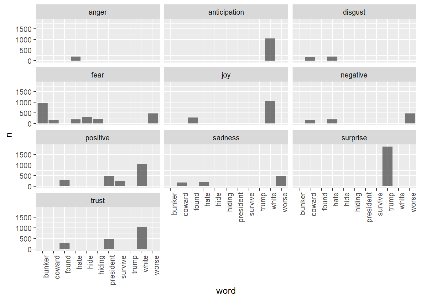
mis_tokens_afinn <- mis_tokens %>%
select(id, retweetCount, favoriteCount, created, retweetCount, isRetweet,
word) %>%
inner_join(get_sentiments("afinn")) ## Joining, by = "word"mis_tokens_afinn %>%
group_by(id, created) %>%
summarize(sentiment = mean(value)) %>%
ggplot(aes(x = created, y = sentiment)) +
geom_smooth(method = loess, formula = y ~ x) +
labs(x = "Date", y = "Media usando Afinn")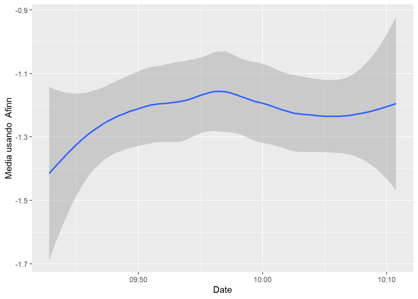
4.4.3 Text Mining Ciberseguridad
library(tm)
library(pdftools)
library(stringr)
library(stringi)
#Depende de Sistema operativo
directorio.textos <- file.path("./","cybersecurity_pdfs")
#directorio.textos <- file.path("C:", "texts")
directorio.textos## [1] ".//cybersecurity_pdfs"## [1] "Accenture-Cybersecurity-Report-2020.pdf"
## [2] "ACS_Cybersecurity_Guide.pdf"
## [3] "An-Introduction-to-Cyber-Security.pdf"
## [4] "cyberplanner.pdf"
## [5] "cybersecuirty_sb_factsheets_all.pdf"
## [6] "Cybersecurity_Guide_For_Dummies_Compressed.pdf"
## [7] "CybersecurityBestPracticesGuide_en.pdf"
## [8] "DETECT AND PREVENT WEB SHELL MALWARE.PDF"
## [9] "ecs-cppp-sria.pdf"
## [10] "ESET_Trends_Report_2019.pdf"
## [11] "ey-cybersecurity-regained-preparing-to-face-cyber-attacks.pdf"
## [12] "G7_Fundamental_Elements_Oct_2016.pdf"
## [13] "GAC16_Cybersecurity_WhitePaper_.pdf"
## [14] "Overviewofcybersecurity.pdf"
## [15] "study_eucybersecurity_en.pdf"#Leer los nombres de los ficheros
list.files <- DirSource(directorio.textos)
# Si es un fichero de texto
# docs <- Corpus(DirSource(directorio.textos))
texts <- lapply(list.files, pdf_text)
length(texts)## [1] 6# No muestro los textos pues tarda en ejecutarse bastante
# texts
# texts[1]
# Obtenemos las logintudes de cada uno
lapply(texts, length) ## $encoding
## [1] 48
##
## $length
## [1] 72
##
## $position
## [1] 10
##
## $reader
## [1] 51
##
## $mode
## [1] 24
##
## $filelist
## [1] 34## <<VCorpus>>
## Metadata: corpus specific: 0, document level (indexed): 0
## Content: documents: 6to_TDM <- function(my_corpus){
my_tdm <- TermDocumentMatrix(my_corpus,
control =
list(removePunctuation = TRUE,
stopwords = TRUE,
tolower = TRUE,
stemming = FALSE,
removeNumbers = TRUE,
bounds = list(global = c(3, Inf))))
}
# Conversion a termDocumentMatrix
my_tdm <- to_TDM(my_corpus)
inspect(my_tdm[1:20,])## <<TermDocumentMatrix (terms: 20, documents: 6)>>
## Non-/sparse entries: 87/33
## Sparsity : 28%
## Maximal term length: 10
## Weighting : term frequency (tf)
## Sample :
## Docs
## Terms 1 2 3 4 5 6
## able 7 5 1 6 3 5
## access 6 21 5 85 21 15
## according 1 9 0 1 0 9
## account 2 2 1 18 7 6
## accounts 0 9 5 9 1 5
## across 11 4 0 2 0 0
## act 0 4 0 6 1 5
## action 11 1 2 18 1 2
## activities 1 0 0 8 2 4
## activity 2 1 0 5 1 8## --------------------------------------------------------
my_corpus <- tm_map(my_corpus, removePunctuation, ucp = TRUE)
# eliminar espacios en blanco
my_corpus <- tm_map(my_corpus,stripWhitespace)
my_corpus <- tm_map(my_corpus,content_transformer(tolower))
# my_corpus <- tm_map(my_corpus,removeNumbers)
# my_corpus <- tm_map(my_corpus,removeWords,my.stopwords)
# my_corpus <- tm_map(my_corpus,removePunctuation)
# my_corpus <- tm_map(my_corpus,stripWhitespace)
# Eliminar palabras individuales
my_corpus <- tm_map(my_corpus, removeWords, c("will", "use", "can"))
# Eliminaciones adicionales
my_corpus <- tm_map(my_corpus, removeWords, c("may", "one"))
my_corpus <- tm_map(my_corpus, removeWords, stopwords("english"))
# prueba paso a paso para ver la estructura
# my_corpus[1]$content$encoding$content
my_tdm <- to_TDM(my_corpus)
inspect(my_tdm[1:20,])## <<TermDocumentMatrix (terms: 20, documents: 6)>>
## Non-/sparse entries: 88/32
## Sparsity : 27%
## Maximal term length: 10
## Weighting : term frequency (tf)
## Sample :
## Docs
## Terms 1 2 3 4 5 6
## able 7 5 1 6 3 5
## access 6 21 5 85 21 15
## according 1 9 0 1 0 9
## account 2 2 1 18 7 6
## accounts 0 9 5 9 1 5
## across 11 4 0 2 0 0
## act 0 4 0 6 1 5
## action 11 2 2 18 1 2
## activities 1 1 0 8 2 4
## activity 2 1 0 5 1 8## Esto seria otra forma de elaborar el corpus, como se hace por ejemplo en el text mining de tweets
## ---- eval=FALSE-----------------------------------------
## toSpace <- content_transformer(function (x , pattern ) gsub(pattern, " ", x))
## corpus <- tm_map(corpus, toSpace, "\n")
## corpus <- tm_map(corpus, toSpace, "<d5>")
## corpus <- tm_map(corpus, toSpace, "<d1>")
## corpus <- tm_map(corpus, toSpace, "\f")
##
## #inspect(corpus[1]);inspect(corpus[2])
##
## --------------------------------------------------------
frequent_terms <- findFreqTerms(my_tdm,
lowfreq = 100,
highfreq = Inf)
frequent_terms## [1] "access" "also" "attack" "attacks"
## [5] "breaches" "business" "company" "computer"
## [9] "cyber" "cybersecurity" "data" "devices"
## [13] "email" "employees" "information" "internet"
## [17] "make" "network" "security" "small"
## [21] "software" "technology" "threats" "web"## --------------------------------------------------------
matrix_tdm <- as.matrix(my_tdm[frequent_terms,])
matrix_tdm## Docs
## Terms 1 2 3 4 5 6
## access 6 21 5 85 21 15
## also 10 43 13 79 7 22
## attack 18 48 4 23 14 40
## attacks 43 41 0 17 7 17
## breaches 73 10 3 17 2 1
## business 25 35 5 131 79 3
## company 3 15 1 52 21 17
## computer 0 24 2 53 20 22
## cyber 43 59 39 96 19 9
## cybersecurity 84 184 0 4 39 20
## data 14 98 17 180 53 29
## devices 0 44 5 41 29 24
## email 0 10 6 62 66 16
## employees 1 3 0 81 21 0
## information 8 43 30 227 45 52
## internet 0 42 1 46 4 29
## make 4 15 1 36 42 17
## network 3 24 1 57 47 23
## security 140 103 48 209 40 28
## small 0 4 1 81 26 2
## software 2 24 15 72 24 2
## technology 14 64 5 12 7 6
## threats 9 84 5 16 5 13
## web 0 15 2 90 12 9Vamos a generar algunas visualizaciones con wordcloud
## Loading required package: RColorBrewer# Tiene que ser la traspuesta, pues my_tdm tiene como nombre de columnas el numero del documento. A nosotros nos interesa que las columans representen la palabra y asi poder calcular su suma. Tambien podriamos haber aplicado rowSums.
freq <- colSums(t(as.matrix(my_tdm)))
set.seed(142)
wordcloud(names(freq), freq, max.words=60, rot.per=0.2, colors=brewer.pal(6, "Paired"))
wordcloud(names(freq), freq, scale=c(3,0.5), max.words=60, random.order=FALSE,
rot.per=0.10, use.r.layout=TRUE, colors=brewer.pal(6, "Dark2")) 
Analisis de sentimientos.
Siguiendo el analsis del siguiente enlance:
https://www.tidytextmining.com/dtm.html
La función inner_join() añade la información de sentimiento de esa palabra.
library(tidytext)
library(dplyr)
library(ggplot2)
terms <- Terms(my_tdm)
ap_td <- tidy(t(my_tdm))
ap_td## # A tibble: 4,668 x 3
## document term count
## <chr> <chr> <dbl>
## 1 1 ability 5
## 2 1 able 7
## 3 1 access 6
## 4 1 according 1
## 5 1 account 2
## 6 1 accurately 2
## 7 1 achieve 11
## 8 1 across 11
## 9 1 action 11
## 10 1 actions 1
## # ... with 4,658 more rows## # A tibble: 528 x 4
## document term count sentiment
## <chr> <chr> <dbl> <chr>
## 1 1 accurately 2 positive
## 2 1 advanced 9 positive
## 3 1 advantage 9 positive
## 4 1 attack 18 negative
## 5 1 attacks 43 negative
## 6 1 bad 1 negative
## 7 1 benefit 13 positive
## 8 1 benefits 3 positive
## 9 1 best 10 positive
## 10 1 better 25 positive
## # ... with 518 more rowsap_sentiments %>%
summarise(Negative = sum(sentiment == "negative"),
positive = sum(sentiment == "positive"))## # A tibble: 1 x 2
## Negative positive
## <int> <int>
## 1 253 275ap_sentiments %>%
count(sentiment, term, wt = count) %>%
ungroup() %>%
filter(n >= 50) %>%
mutate(n = ifelse(sentiment == "negative", -n, n)) %>%
mutate(term = reorder(term, n)) %>%
ggplot(aes(term, n, fill = sentiment)) +
geom_bar(stat = "identity") +
ylab("Contribution to sentiment") +
coord_flip()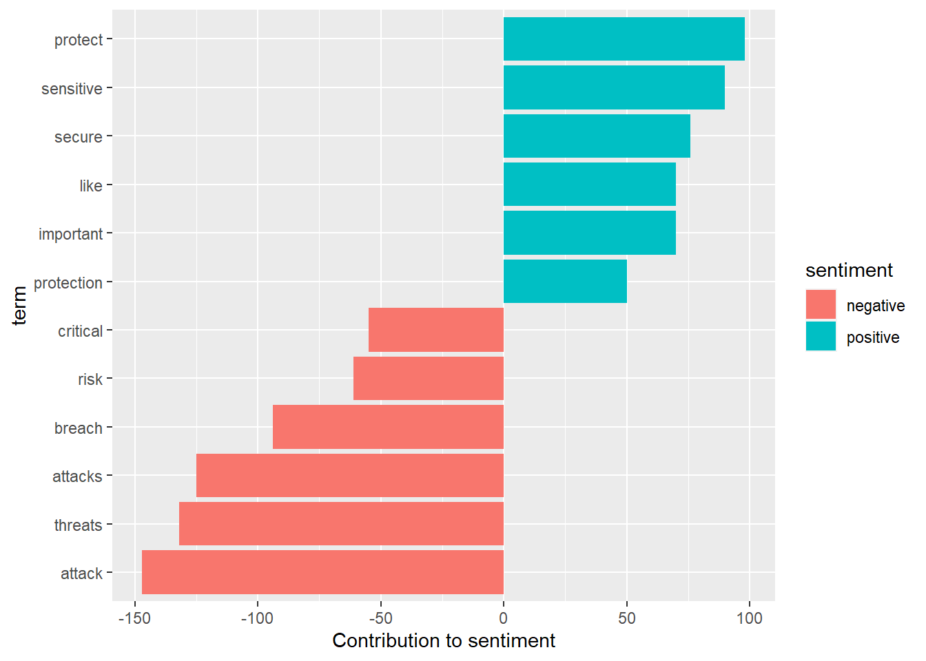
A partir de aqui es una adaptacion del tutorial visto en clase para el analisis de tweets con tidytext
O en el mismo gráfico juntamos los sentimientos positivos y negativos:
ap_sentiments %>%
count(sentiment, term, wt = count) %>%
ungroup() %>%
filter(n>50) %>%
mutate(n = ifelse(sentiment == "negative", -n, n)) %>%
ggplot(aes(term, n, fill = sentiment)) + geom_col() + coord_flip() +
ggtitle("Contribución al sentimiento") +
theme_minimal()