Chapter 5 More complex models
This will include logistic regression, as well as potentially more models as time allows! Packages introduced: forcats, stringr.
5.1 Wrapping up linear regression
I have given you a crash course in linear regression, although there are of course many topics we couldn’t even touch on!
- transformations
- outliers and their influence
- ANOVA
- prediction/confidence intervals for particular values
- variable selection methods
- colinearity / multicolinearity
- model selection methods
- and much more!
I have playlists for my STAT 320 course that cover many of these topics.
Linear regression is useful because it can be applied to many different problems. The topics in an introductory statistics course are often taught as distinct methods (inference for one mean, inference for a difference of means, inference for many means, etc) but they can all be done as linear models!
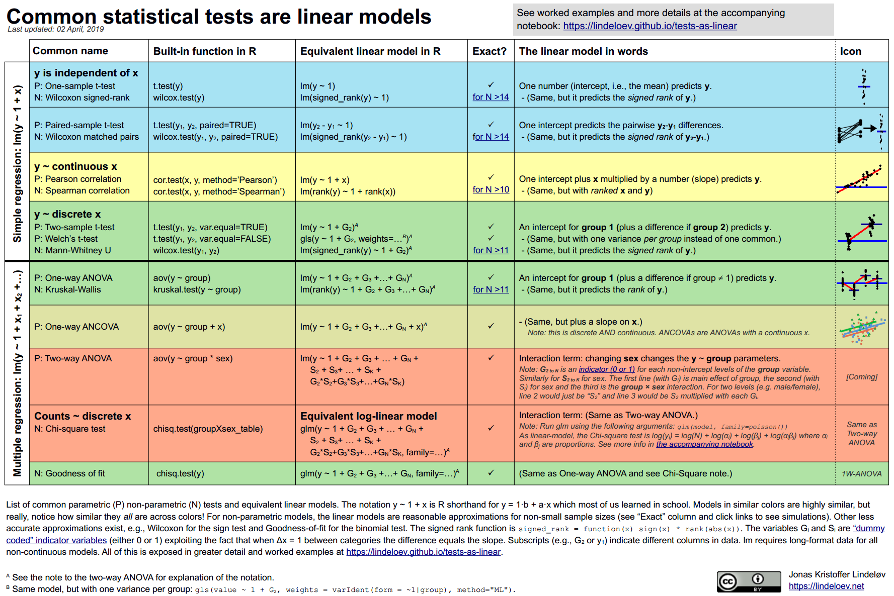
This cheatsheet comes from the awesome website, Common statistical tests are linear models (or: how to teach stats) and includes R code, theory, and examples. They also link to a python version!
5.2 Logistic regression
For all it’s flexibility, linear regression essentially only works for a quantitative response variable. Sometimes, we want to model a response variable that is binary, meaning that it can take on only two possible outcomes. These outcomes could be labeled “Yes” or “No”, or “True” or “False”, but are things that can be coded as either 0 or 1. We have seen these types of variables before (as indicator variables), but we always used them as explanatory variables. Creating a model for such a variable as the response requires a more sophisticated technique than ordinary least squares regression. It requires the use of a logistic model.
Instead of modeling \(\pi\) (the response variable) like this, \[ \pi = \beta_0 + \beta_1 X \]
suppose we modeled it like this, \[ \log \left( \frac{\pi}{1-\pi} \right) = logit(\pi) = \beta_0 + \beta_1 X \] This transformation is called the logit function. Note that this implies that \[ \pi = \frac{e^{\beta_0 + \beta_1 X}}{1 + e^{\beta_0 + \beta_1 X}} \in (0,1) \]
The logit function constrains the fitted values to lie within \((0,1)\), which helps to give a natural interpretation as the probability of the response actually being 1.
Logistic regression:
- uses logit function as a “link”
- logit produces an S-curve inside [0,1]
- fit using maximum likelihood estimation, not minimizing the sum of the squared residuals
- really, no residuals! This means we don’t have sums of squares
Let’s think about an example. I have some data about NFL field goals. This came from a website of miscellaneous datasets. You can read about the data here and download it here (may just download if you click).
library(readr)
library(dplyr)
library(broom)
library(ggplot2)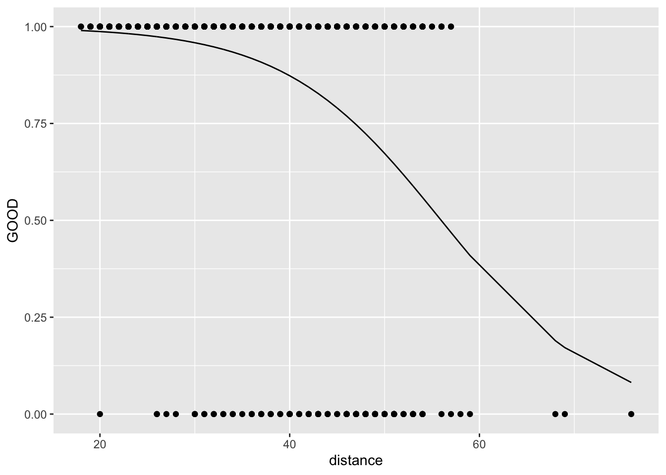
football <- read_csv("data/nfl2008_fga.csv")It would be bad practice to fit
lm1 <- lm(GOOD~distance, data = football)
ggplot(football, aes(x = distance, y = GOOD)) +
  geom_point() +
  geom_smooth(method="lm", se = FALSE)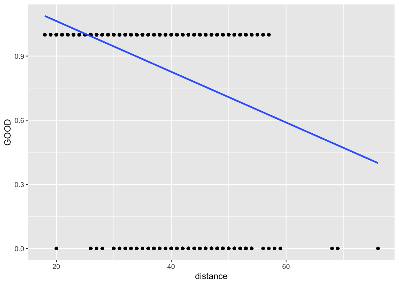
Instead, we should fit
This model is more complicated than the other ones we’ve seen.
5.3 “Spaces”
In logistic regression, we think in three different “spaces”
- log-odds space
- odds space
- probability space
5.3.1 Log-odds space
Logistic regression is linear in log-odds space.
Why is this useful?
5.3.2 Odds space
\[ \frac{\pi}{1-\pi} = e^{\beta_0+\beta_1\cdot X} \]
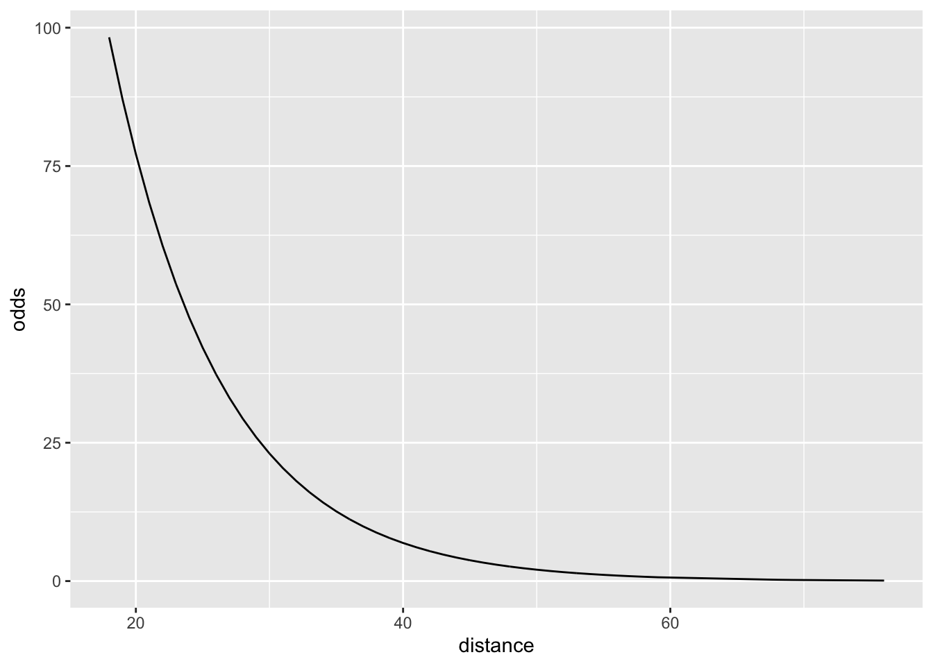
Why is this useful?
5.3.3 Probability space
\[ \pi = \frac{e^{\beta_0+\beta_1\cdot X}}{1+e^{\beta_0+\beta_1\cdot X}} \]
Why is this useful?
5.4 Fitting a logistic model
Fitting a logistic curve is mathematically more complicated than fitting a least squares regression, but the syntax in R is similar, as is the output. The procedure for fitting is called maximum likelihood estimation, and the usual machinery for the sum of squares breaks down. Consequently, there is no notion of \(R^2\), etc.
Instead of using lm() to model this kind of response, we use glm() with the argument family=binomial
- How can we interpret the coefficients of this model in the context of the problem?
The interpretation of the coefficients in a linear regression model are clear based on an understanding of the geometry of the regression model. We use the terms intercept and slope because a simple linear regression model is a line. In a simple logistic model, the line is transformed by the logit function. How do the coefficients affect the shape of the curve in a logistic model?
I have created a shiny app that will allow you to experiment with changes to the intercept and slope coefficients in the simple logistic model for isAlive as a function of age.
- How do changes in the intercept term affect the shape of the logistic curve?
- How do changes in the slope term affect the shape of the logistic curve?
5.4.1 Interptetation
\(\beta_1\) is the typical change in the log-odds for each one-unit increase in x.
\(e^{\beta_1}\) is the multiplier for odds for each one-unit increase.
These changes are constant
5.5 Visualizing the model
Like we did with linear regression, the broom package can do the work of tidying up our model objects for us.
- What variables are in this new dataset?
- What does the
data=argument do?
- What does this
mutate()code do?
5.6 Binning
In order to plot data points in those spaces, it can be useful to bin the explanatory variable and then compute the average proportion of the response within each bin.
football <- football %>%
  mutate(distGroup = cut(distance, breaks = 10))
football %>%
  group_by(distGroup) %>%
  skim(GOOD)
football_binned <- football %>%
group_by(distGroup) %>%
summarize(binnedGOOD = mean(GOOD), binnedDist = mean(distance)) %>%
mutate(logit = log(binnedGOOD/(1-binnedGOOD)))- What does this code do?
- How many observations are in our new dataset?
Then, it can be illustrative to see how the logistic curve fits through this series of points.
ggplot(football_binned) +
geom_point(aes(x = binnedDist, y = binnedGOOD)) +
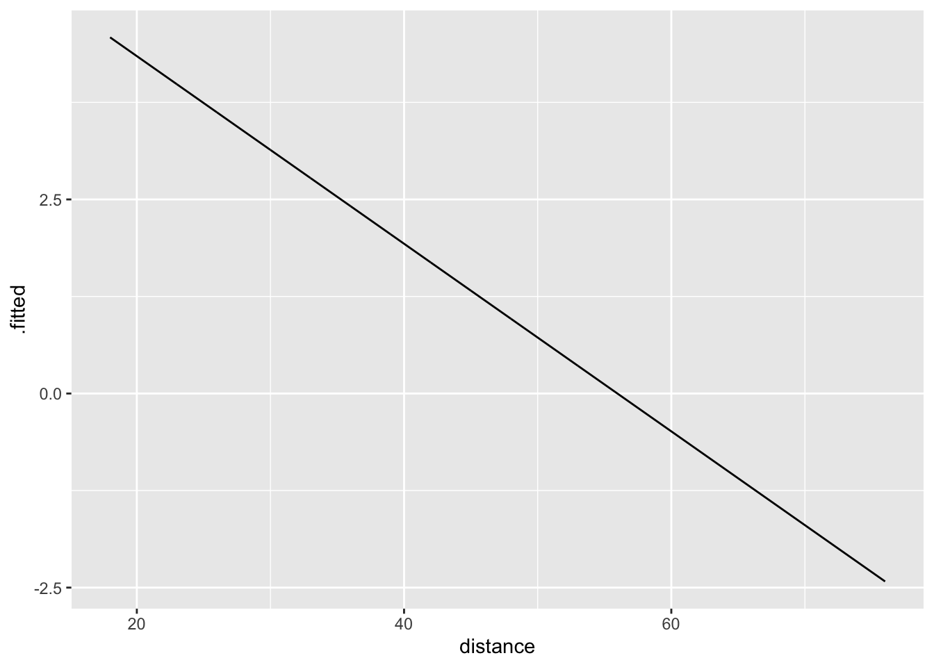
geom_line(data = football_logm1, aes(x = distance, y = probability))Consider now the difference between the fitted values and the link values. Although the fitted values do not follow a linear pattern with respect to the explanatory variable, the link values do. To see this, let’s plot them explicitly against the logit of the binned values.
ggplot(football_binned) +
  geom_point(aes(x = binnedDist, y = logit)) +
  geom_line(data = football_logm1, aes(x = distance, y = .fitted))
Note how it is considerably easier for us to assess the quality of the fit visually using the link values, as opposed to the binned probabilities.
- Why can’t we take the logit of the actual responses?
5.7 Checking conditions
Of course, we have conditions that are necessary to use a logistic model for inference. These are similar to the requirements for linear regression:
- Linearity of the logit (or \(\log{(odds)}\))
- Independence
- Random
The requirements for Constant Variance and Normality are no longer applicable. In the first case, the variability in the response now inherently depends on the value, so we know we won’t have constant variance. In the second case, there is no reason to think that the residuals will be normally distributed, since the “residuals” are can only be computed in relation to 0 or 1. So in both cases the properties of a binary response variable break down the assumptions we made previously.
Let’s look at the empirical logit plot again.
ggplot(football_binned) +
  geom_point(aes(x = binnedDist, y = logit)) +
geom_line(data = football_logm1, aes(x = distance, y = .fitted))- Does it look like the linearity condition is upheld?
5.8 Comparing to a null model
We’d like to consider how well this model is working by looking at its predictions, and comparing them to a null model. The most boring prediction we could use is the mean,
If we used the average as our prediction, we would predict that every kick was good, and we would be right 87% of the time. So, we’d like to do even better than that with our model.
One technique for assessing the goodness-of-fit in a logistic regression model is to examine the percentage of the time that our model was “right.” What does it mean to be correct in this situation? The response variable is binary, but the predictions generated by the model are quantities on \([0,1]\). A simple way to classify the fitted values of our model is to simply round them off. Once we do this, we can tabulate how often the rounded-off probability from the model agrees with the actual response variable.
- How many observations did we correct? How many incorrect?
- Are we doing better than just using the mean?
Of course, there are many more sophisticated ways to assess a logistic regression model.
5.9 Multiple logistic regression
Just as with linear regression, we can use arbitrarily many predictors in our logistic regression model.
Try generating a model with multiple predictor variables.
Is it better than the simple logistic model? How can you tell?
5.10 strings and factors
Sometimes you have messy character strings in your data, and you want to do something with them. The package stringr has lots of utilities, but even more often when I reach for that package I want the separate function from the tidyr package.
Let’s look at the RailsTrails dataset. This is technically data(RailsTrails, package = "Stat2Data"), but again, I wrote it out to a .csv to give you more practice downloading and importing data. It is available on my GitHub.
Maybe we want to know about the suffixes (?) of the street names. In other words, are they St, Dr, etc? Let’s use separate to pull that variable apart into two.
RailsTrails %>%
  separate(StreetName, into = c("name", "kind"),
           sep = " ", remove = FALSE, extra = "merge") %>%
  select(StreetName, name, kind)
this isn’t quite what we wanted. Weird! Like I said, separate is the solution to many woes.
Today, we need to do something a little more complicated. Let’s try a stringr function.
library(purrr)
RailsTrails %>%
  mutate(pieces = str_split(StreetName, " ")) %>%
  select(StreetName, pieces) %>%
  mutate(last_piece = map_chr(pieces, ~ .x[length(.x)]))
Eek, that one is pretty complicated! Let’s try something a little simpler,
RailsTrails %>%
  mutate(last_piece = word(StreetName, start = -1)) %>%
  select(StreetName, last_piece)
Okay, that looks like what we want.
Finally, we might want to fix up the strings so they are more consistent,
library(forcats)
RailsTrails <- RailsTrails %>%
  mutate(last_piece = as_factor(last_piece)) %>%
  mutate(last_piece = fct_recode(last_piece,
    `Drive` = "Dr",
    `Road` = "Rd",
    `Street` = "St",
    `Drive` = "Dr.",
    `Road` = "Rd.",
    `Avenue` = "Ave"
  ))
ggplot(RailsTrails) +
  geom_bar(aes(x = last_piece))
What if we want the barchart in order of frequency?
RailsTrails <- RailsTrails %>%
  mutate(last_piece = fct_infreq(last_piece))
ggplot(RailsTrails) +
  geom_bar(aes(x = last_piece))
As a last activity, let’s try making a logistic regression model to predict if a house in Northampton, MA has a garage.
We’ll need to do a little more data cleaning before we can do that, because R wants a binary variable for the response, and GarageGroup is currently a character variable.
Now, we can make a model. Perhaps try using that last_piece as a predictor.
5.11 More models
I don’t think we’ll have time to go further than logistic regression today. But, there are extensions to models like this that allow you to do classification on a response that has more than two possibilities. Hopefully, you’ll do some of those classification models next month!
If you’d like to learn more about models from a statistical perspective, try Friedman et al. (2001) or the undergrad version, James et al. (2013). The R code in those books is pretty outdated (hopefully it will be updated in the new editions!) but some colleagues and I have taken a stab at modernizing it, as well as translating it to python, here.
References
Friedman, Jerome, Trevor Hastie, Robert Tibshirani, and others. 2001. The Elements of Statistical Learning. Vol. 1. 10. Springer series in statistics New York.
James, Gareth, Daniela Witten, Trevor Hastie, and Robert Tibshirani. 2013. An Introduction to Statistical Learning. Vol. 112. Springer.