Chapter 8 Visualizing and characterizing variability

[This “chapter” is essentially the same as 2, but with some of the notes I wrote in the document as we went.]

This workshop will attempt to teach you some of the basics of the data science workflow, as imagined by Wickham and Grolemund:

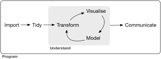
via Wickham and Grolemund (2017)

Notice that this graphic already includes a cycle– this is an important part of the process! It is unlikely (impossible) that you could work linearly through a data science project.

It is tempting to focus on the modeling aspect of the cycle, and miss the other elements. But, recall

“90% of data science is wrangling data, the other 10% is complaining about wrangling data.”@evelgab at #rstatsnyc

— David Robinson (@drob) April 20, 2018

Statistics is the practice of using data from a sample to make inferences about some broader population of interest. Data is a key word here. In the pre-bootcamp prep, you explored the first simple steps of a statistical analysis: familiarizing yourself with the structure of your data and conducting some simple univariate analyses.

We are doing all our work in the programming language R, and I am going to show you one way to do the tasks. However, one of the powers of R is that there are many ways to “say” the same thing in R. In fact, part of my research is about studying the various syntaxes in R (sometimes called Domain Specific Languages). I characterize the three main syntaxes as:

• base R. If you have used R before, it is highly likely you have seen this syntax before. I don’t use it much (anymore). This syntax is characterized by dollar signs $ and square brackets [ , ].
• formula syntax. We will be using this syntax for modeling, but you can also do many other tasks in it, using mosaic for statistics, and then lattice of ggformula graphics
• tidyverse syntax. This is most of what I use for data wrangling and data visualization. Main packages include ggplot2 and dplyr. You can use the convenience package tidyverse to install and load many of the packages.

If you want to see a comparison between these three syntaxes, see my cheatsheet in the “contributed” section of the RStudio Cheatsheets page.

8.1 Pre-bootcamp review

1. What did you learn about hiphop_cand_lyrics?

2. Did exploring the hiphop_cand_lyrics dataset raise any questions for you?

3. What was the variability like in the salary variable in the Salaries dataset?

4. What do you think might explain the variability in salary?

We are going to try to use plots and models to explain this variability.

8.1.1 Variable types, redux

It may be useful to think about variables as

• response variable: this is the one we’re the most interested in, which we think might “respond.”
• explanatory variable(s): these are the ones we think might “explain” the variation in the response.

Before building any models, the first crucial step in understanding relationships is to build informative visualizations.

8.1.2 Visualizing variability (in breakout rooms)

Run through the following exercises which introduce different approaches to visualizing relationships. In doing so, for each plot:

• examine what the plot tells us about relationship trends & strength (degree of variability from the trend) as well as outliers or deviations from the trend.
• think: what’s the take-home message?

We’ll do the first exercise together.

You (hopefully!) need to re-load the Salaries dataset. (If you don’t, that probably means you saved your workspace the last time you closed RStudio, talk to me or a TA about how to clear your workspace.)

library(car)
data(Salaries)

1. Sketches How might we visualize the relationships among the following pairs of variables? Checking out the structure on just a few people might help:

##         rank discipline yrs.since.phd yrs.service    sex salary
## 1       Prof          B            19          18   Male 139750
## 2       Prof          B            20          16   Male 173200
## 3   AsstProf          B             4           3   Male  79750
## 4       Prof          B            45          39   Male 115000
## 5       Prof          B            40          41   Male 141500
## 6  AssocProf          B             6           6   Male  97000
## 7       Prof          B            30          23   Male 175000
## 8       Prof          B            45          45   Male 147765
## 9       Prof          B            21          20   Male 119250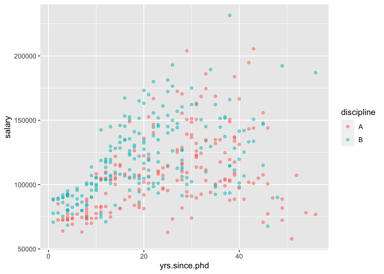
## 10      Prof          B            18          18 Female 129000

1. salary vs. yrs.since.phd (scatterplot, geom_point)
2. salary vs. yrs.service (scatterplot, geom_point)
3. salary vs. discipline (side-by-side boxplots, side-by-histograms)
4. salary vs. yrs.since.phd and discipline (in one plot) (scatterplot with colored dots)
5. salary vs. yrs.since.phd and sex (in one plot) (scatterplot with colored dots)

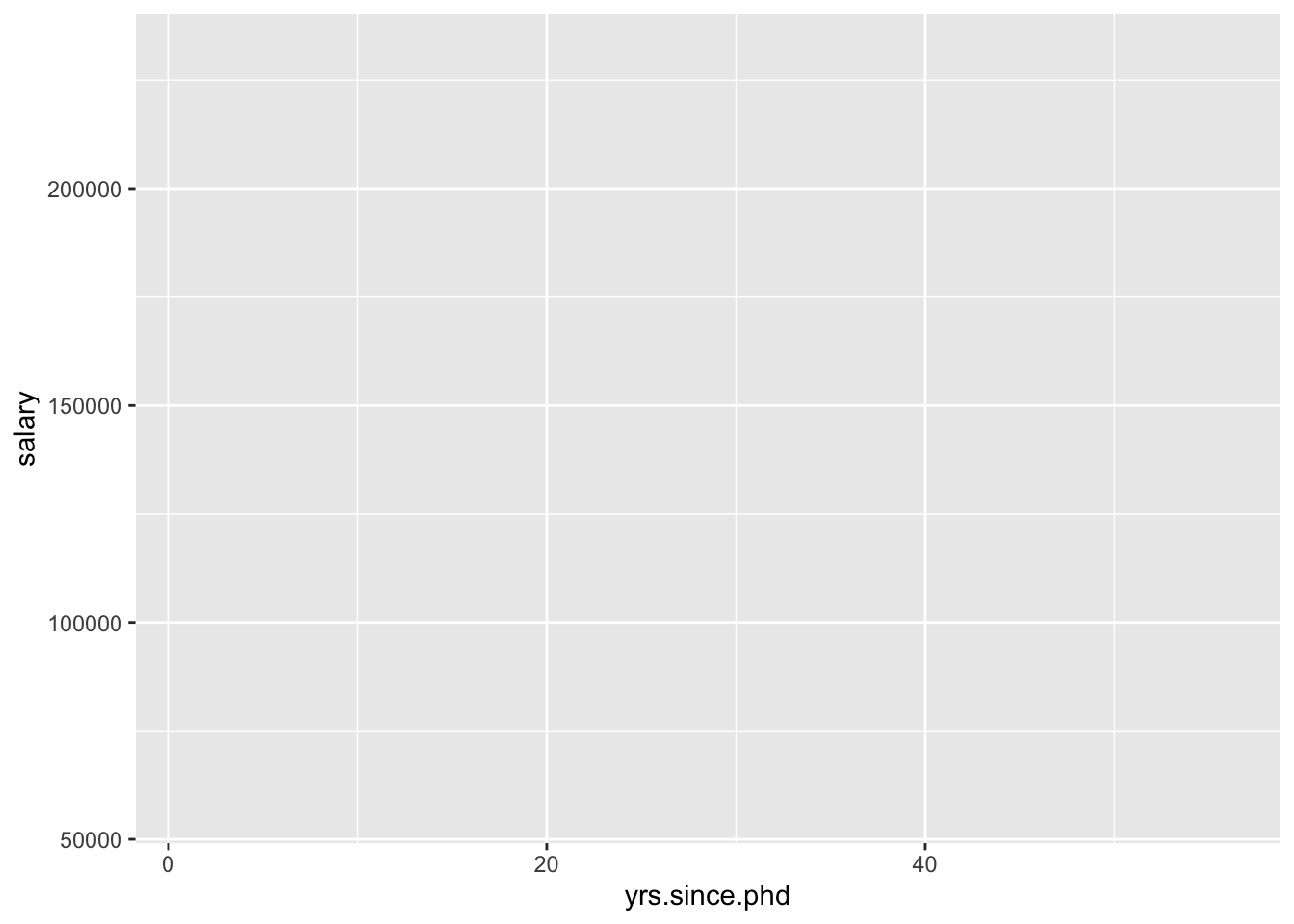
2. Scatterplots of 2 quantitative variables

By default, the response variable (\(Y\)) goes on the y-axis and the predictor (\(X\)) goes on the x-axis.

Again, you (hopefully!) need to re-load ggplot2 in order to run this code.

library(ggplot2)

ggplot(Salaries, aes(x = yrs.since.phd, y = salary))

ggplot(Salaries, aes(x = yrs.since.phd, y = salary)) +
  geom_point()

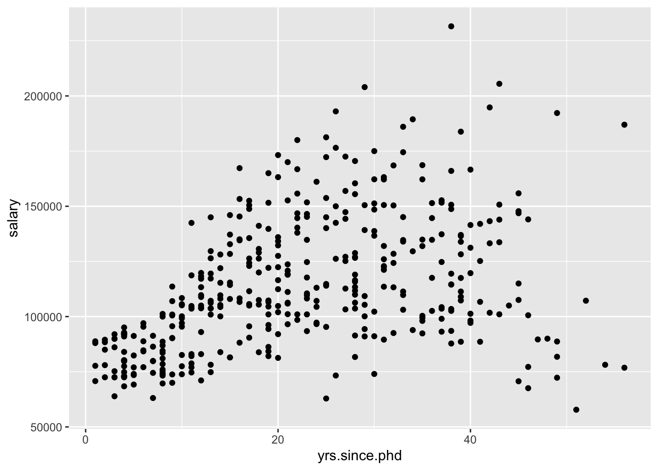
# ggplot(Salaries, aes(x = yrs.since.phd, y = salary)) +
#  geom_text(aes(label = discipline))

# practice: make a scatterplot of salary vs. yrs.service

3. Side-by-side plots of 1 quantitative variable vs. 1 categorical

ggplot(Salaries, aes(x = salary, fill = discipline)) +
  geom_density()

ggplot(Salaries, aes(x = salary, fill = discipline)) +
  geom_density(alpha = 0.5)

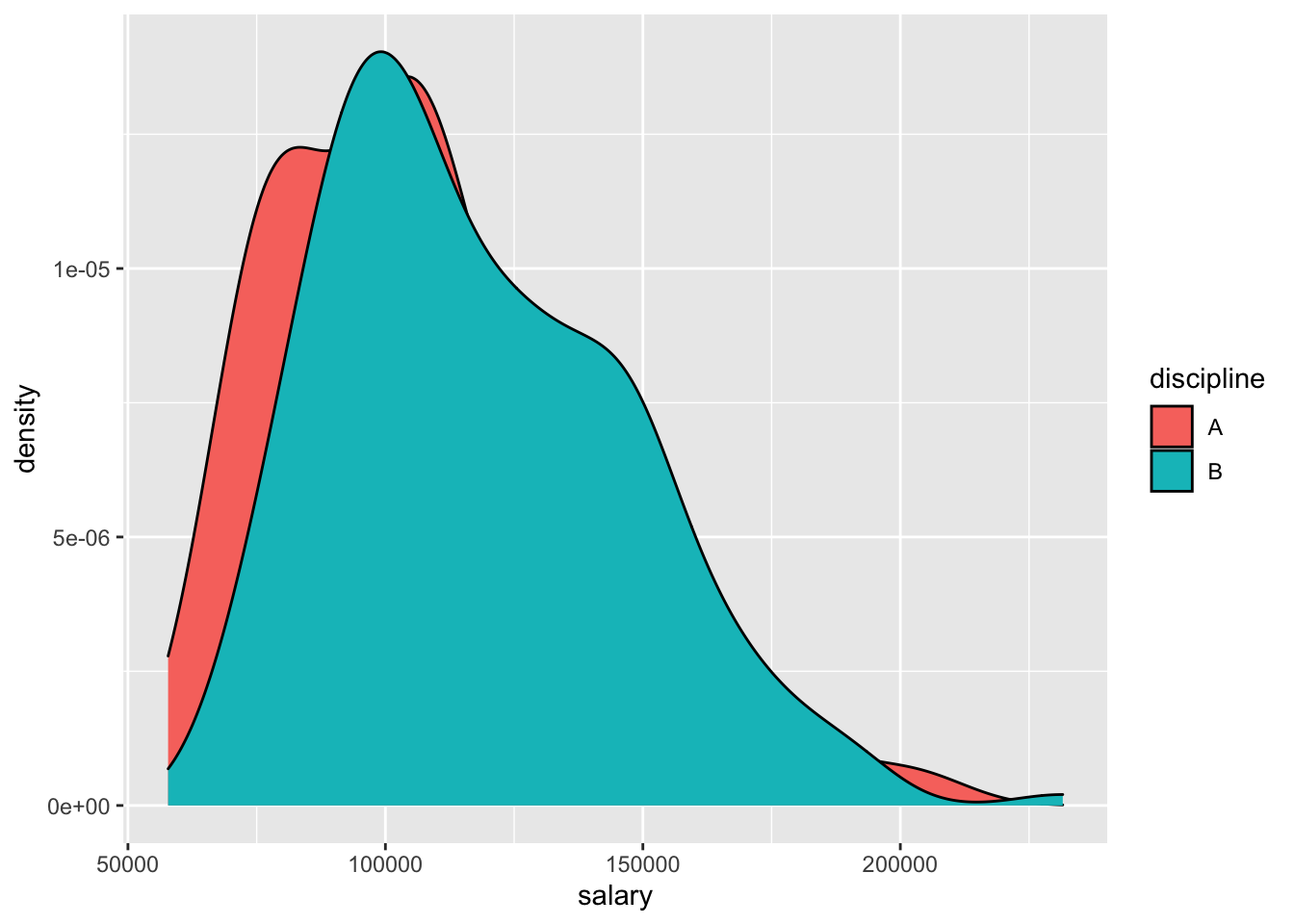
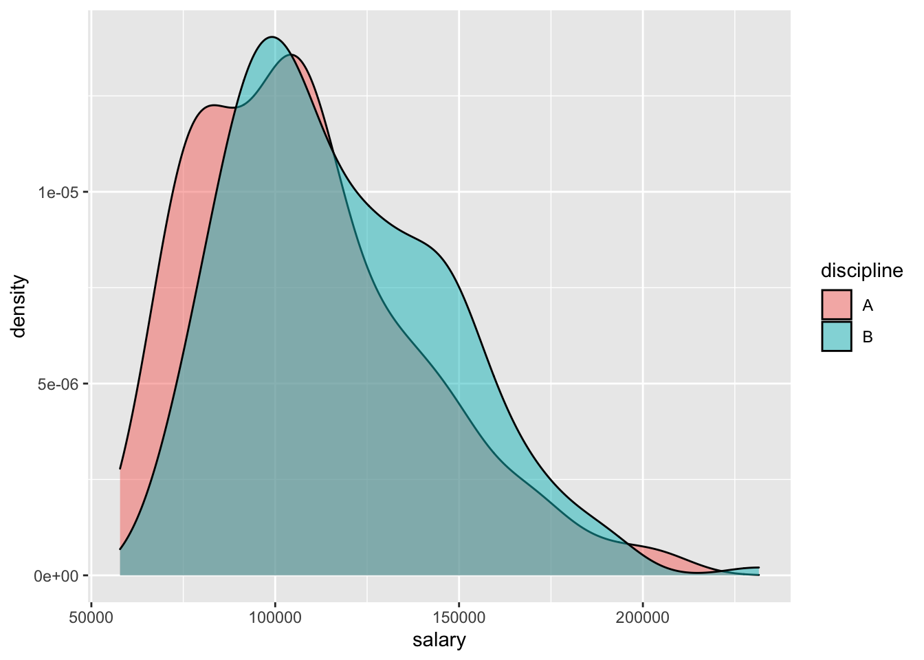
# ggplot(Salaries, aes(x = salary)) +
#   geom_density() +
#   facet_wrap(~discipline)

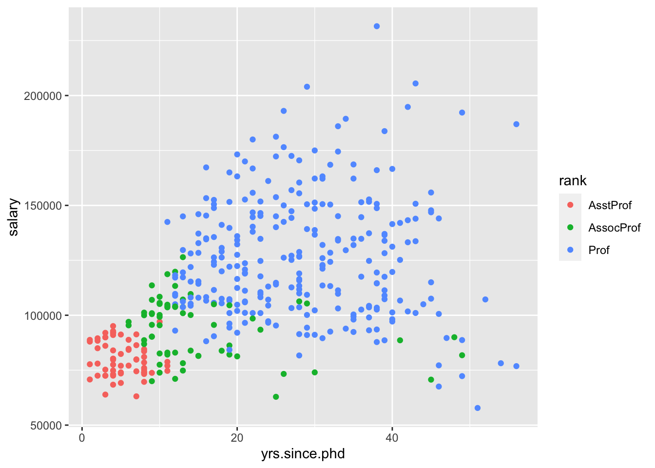
# practice: make side-by-side boxplots of salary by rank

4. Scatterplots of 2 quantitative variables plus a categorical

If yrs.since.phd and discpline both explain some variability in salary, why not look at all the variables at once?

ggplot(Salaries, aes(y = salary, x = yrs.since.phd, color = discipline)) + 
    geom_point(alpha = 0.5)

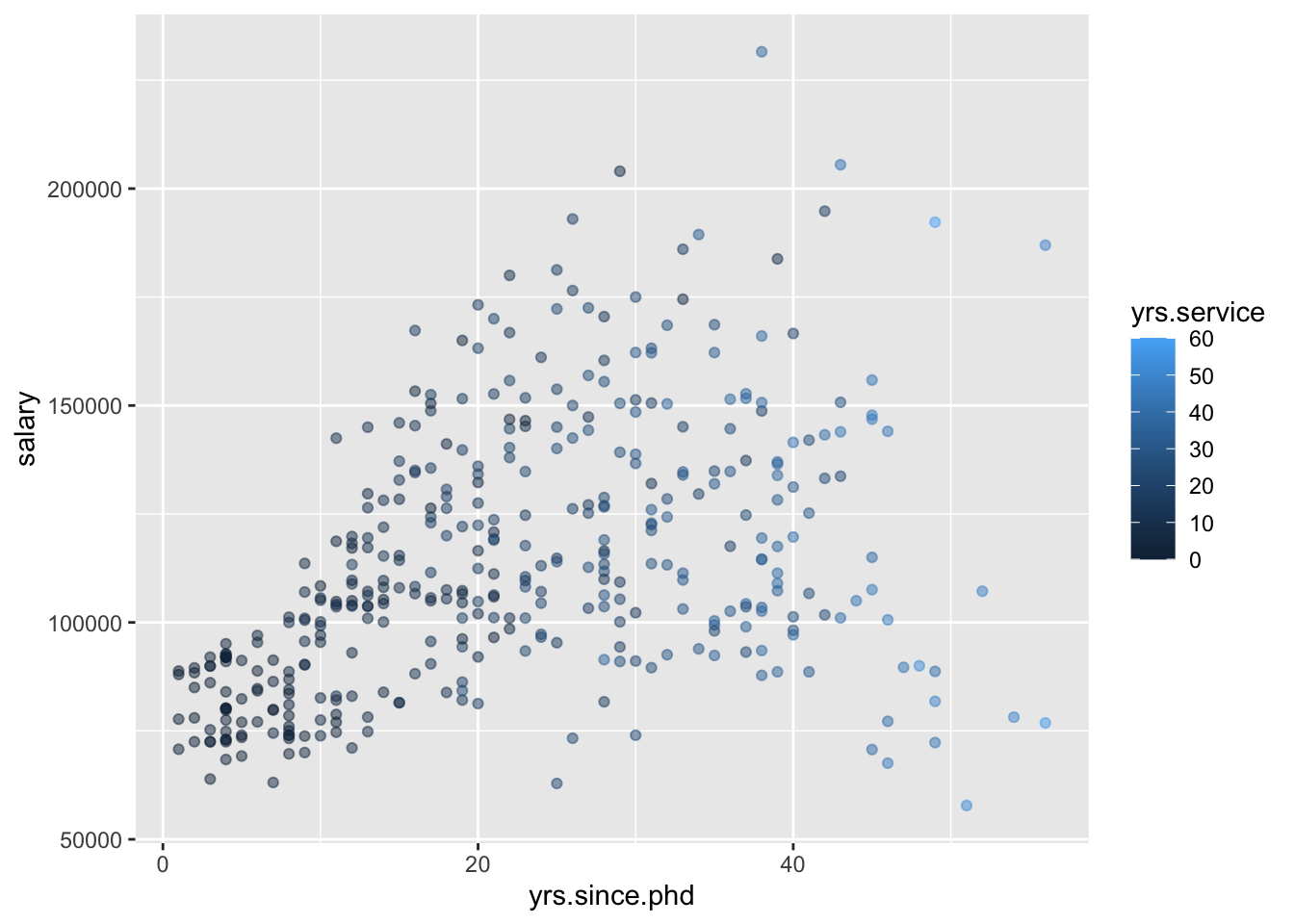
5. Plots of 3 quantitative variables

Think back to our sketches. How might we include information about yrs.service in our plots?

ggplot(Salaries, aes(x= yrs.since.phd, y= salary, color = yrs.service)) +
  geom_point(alpha=0.5)

8.2 Modeling: choose, fit, assess, use

As we look at these pictures, we begin to build mental models in our head. Statistical models are much like mental models (they help us generalize and make predictions) but of course, more rigorous. No matter which model we are using, we will use the CFAU framework,

• Choose
• Fit
• Assess
• Use

We’re going to begin with linear models, which are one of the simplest ways to model.

8.3 Linear models

A linear model is a supervised learning method, in that we will use ground truth to help us fit the model, as well as assess how good our model is.

With regression, your input is

\[ x = (x_1, x_2, \dots, x_k) \] and the output is a quantitative \(y\). We can “model” \(y\) by \(x\) by finding

\[ y = f(x) + \epsilon \]

where \(f(x)\) is some function of \(x\), and \(\epsilon\) are errors/residuals. For simple linear regression, \(f(x)\) will be the equation of a line.

Specifically, we use the notation

\[ Y = \beta_0 + \beta_1\cdot X + \epsilon, \, \epsilon \sim N(0, \sigma_\epsilon) \] although we are primarily concerned with the fitted model,

\[ \hat{Y} = \hat{\beta_0} + \hat{\beta_1}\cdot X \] Notice that there is no \(\epsilon\) in the fitted model. If we want, we can calculate

\[ \epsilon_i = y_i - \hat{y}_i \] for each data point, to get an idea of how “off” the model is.

The coefficients \(\hat{\beta_0}\) and \(\hat{\beta_1}\) are useful for interpreting the model.

\(\hat{\beta_0}\) is the intercept coefficient, the average \(Y\) value when \(X=0\)

\(\hat{\beta_1}\) is the slope, the amount that we predict \(Y\) to change for a 1-unit change in \(X\)

We can use our model to predict \(y\) for new values of \(y\), explain variability in \(y\), and describe relationships between \(y\) and \(x\).

8.4 Linear models in R

The syntax for linear models is different than the tidyverse syntax, and instead is more similar to the syntax for lattice graphics.

The general framework is goal ( y ~ x , data = mydata ) We’ll use it for modeling.

Given how the data looked in the scatterplot we saw above, it seems reasonable to choose a simple linear regression model. We can then fit it using R.

m1 <- lm(salary ~ yrs.since.phd, data = Salaries)

We’re using the assignment operator to store the results of our function into a named object.

I’m using the assignment operator <-, but you can also use =. As with many things, I’ll try to be consistent, but I often switch between the two.

The reason to use the assignment operator here is because we might want to do things with our model output later. If you want to skip the assignment operator, try just running lm(salary ~ yrs.since.phd, data = Salaries) in your console to see what happens.

Now, we want to move on to assessing and using our model. Typically, this means we want to look at the model output (the fitted coefficients, etc). If we run summary() on our model object we can look at the output.

summary(m1)

## 
## Call:
## lm(formula = salary ~ yrs.since.phd, data = Salaries)
## 
## Residuals:
##    Min     1Q Median     3Q    Max 
## -84171 -19432  -2858  16086 102383 
## 
## Coefficients:
##               Estimate Std. Error t value Pr(>|t|)    
## (Intercept)    91718.7     2765.8  33.162   <2e-16 ***
## yrs.since.phd    985.3      107.4   9.177   <2e-16 ***
## ---
## Signif. codes:  0 '***' 0.001 '**' 0.01 '*' 0.05 '.' 0.1 ' ' 1
## 
## Residual standard error: 27530 on 395 degrees of freedom
## Multiple R-squared:  0.1758, Adjusted R-squared:  0.1737 
## F-statistic: 84.23 on 1 and 395 DF,  p-value: < 2.2e-16

The p-values are quite significant, which might lead us to assess that the model is pretty effective.

We could visualize the model using ggplot2, by adding an additional geom_,

ggplot(Salaries, aes(x = yrs.since.phd, y = salary)) +
  geom_point() +
  geom_smooth(method = "lm", se = FALSE)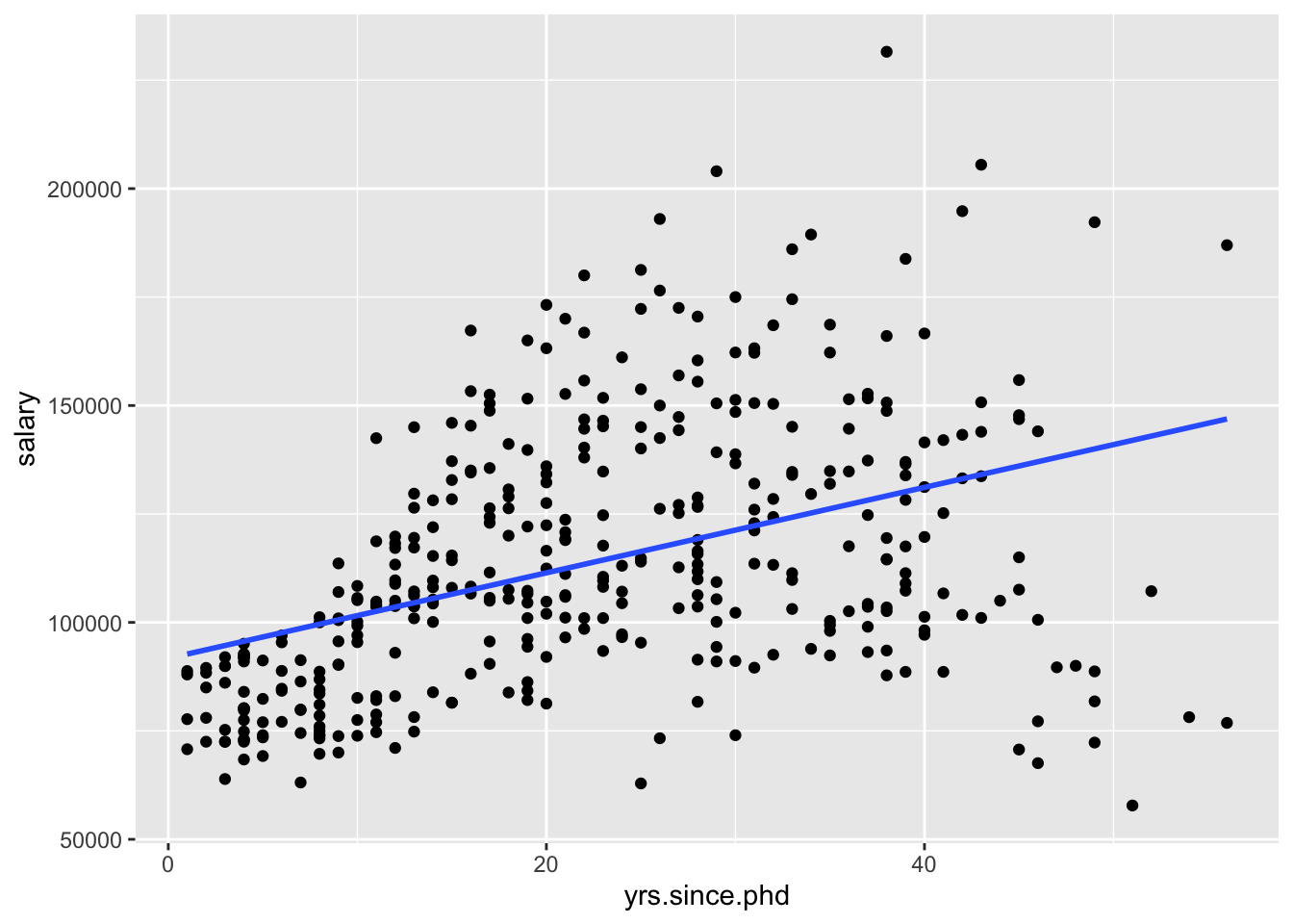

geom_smooth can use other methods, but we want a linear model. And we’ll talk about standard errors eventually, but for now we’ll turn them off.

We can also use the model for description. To write this model out in our mathematical notation,

\[ \widehat{\texttt{salary}} = 91718.7 + 985.3\cdot \texttt{yrs.since.phd} \]

1. What would this model predict for the salary of a professor who had just finished their PhD?

91718.7 + 985.3*0

## [1] 91718.7

We would predict $91,719.

2. What does the model predict for a professor who has had their PhD for 51 years?

91718.7 + 985.3*51

## [1] 141969

We would predict $141,969.

3. What was the observed salary value for the person with 51 years of experience?

Salaries %>%
  filter(yrs.since.phd == 51) %>%
  select(salary)

##   salary
## 1  57800

4. What is the residual?

57800 - 141969

## [1] -84169

To assess further, we can compare it to a “null” model, where we don’t use a predictor (Instead, we just use the mean as the model for every observation).

We can run two models and visualize them to compare! The first is the average, and the second is the least squares regression line. We can think of the latter as a the null model where \(\beta_1 = 0\) and \(\hat{y} = \bar{y}\). Which model do you think is better?

modMean <- lm(salary ~ 1, data = Salaries)
summary(modMean)

## 
## Call:
## lm(formula = salary ~ 1, data = Salaries)
## 
## Residuals:
##    Min     1Q Median     3Q    Max 
## -55906 -22706  -6406  20479 117839 
## 
## Coefficients:
##             Estimate Std. Error t value Pr(>|t|)    
## (Intercept)   113706       1520    74.8   <2e-16 ***
## ---
## Signif. codes:  0 '***' 0.001 '**' 0.01 '*' 0.05 '.' 0.1 ' ' 1
## 
## Residual standard error: 30290 on 396 degrees of freedom

p1 <- ggplot(Salaries, aes(x = yrs.since.phd, y = salary)) + geom_point()

p1 + geom_abline(slope = 0, intercept = 113706)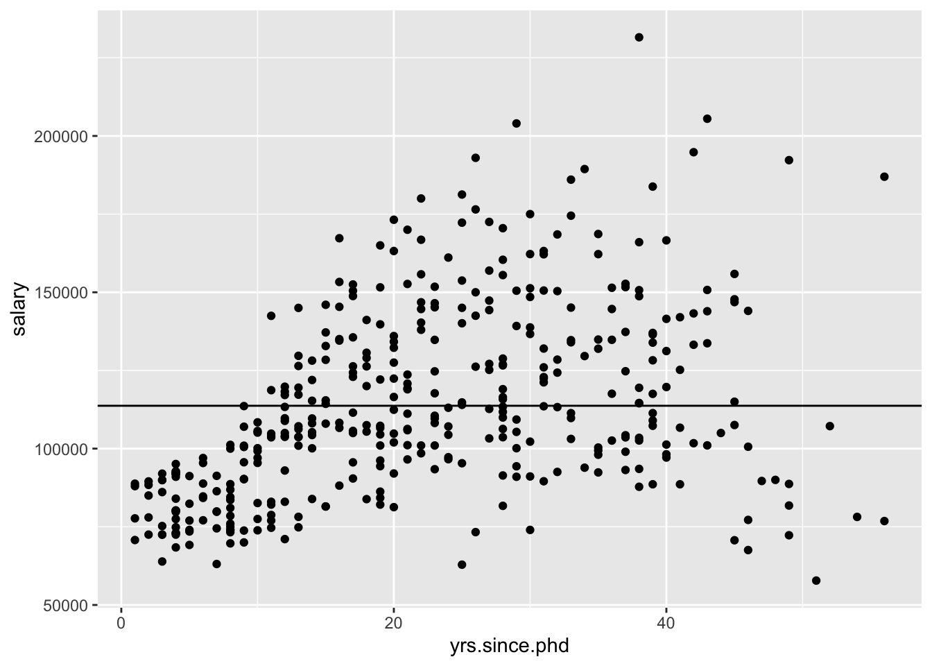

p1 + geom_smooth(method = lm, se = FALSE, color ="red") + geom_abline(slope = 0, intercept = 113706, color = "blue")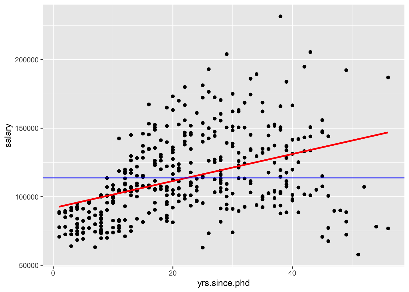

Let’s interpret the slope and intercept:

• “For a 1-unit increase in x, we would expect to see a \(\hat{\beta}_1\)-unit increase/decrease in y.”

• “For a 1-year increase in years since PhD, we would expect to see a 985-dollar increase in salary.”

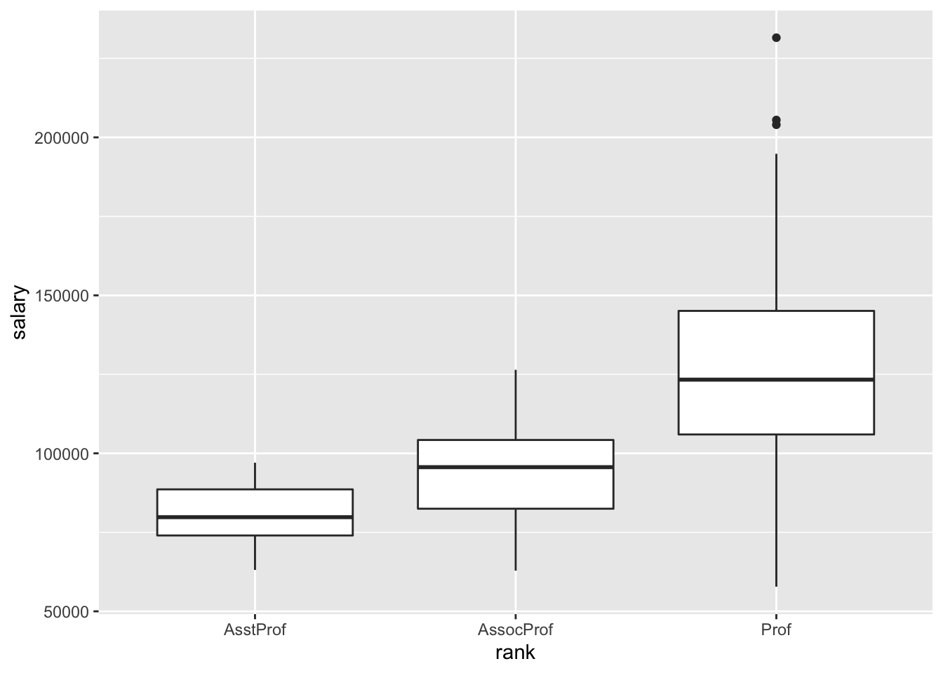
8.4.1 Linear model with one categorical predictor

We thought that rank probably explained some of the variability in salary as well. We could make another simple linear regression model using just rank as a predictor,

m2 <- lm(salary~rank, data=Salaries)

summary(m2)

## 
## Call:
## lm(formula = salary ~ rank, data = Salaries)
## 
## Residuals:
##    Min     1Q Median     3Q    Max 
## -68972 -16376  -1580  11755 104773 
## 
## Coefficients:
##               Estimate Std. Error t value Pr(>|t|)    
## (Intercept)      80776       2887  27.976  < 2e-16 ***
## rankAssocProf    13100       4131   3.171  0.00164 ** 
## rankProf         45996       3230  14.238  < 2e-16 ***
## ---
## Signif. codes:  0 '***' 0.001 '**' 0.01 '*' 0.05 '.' 0.1 ' ' 1
## 
## Residual standard error: 23630 on 394 degrees of freedom
## Multiple R-squared:  0.3943, Adjusted R-squared:  0.3912 
## F-statistic: 128.2 on 2 and 394 DF,  p-value: < 2.2e-16

What is the estimated model formula?

\[ \widehat{salary} = 80776 + 13100\cdot rankAssocProf + 45996\cdot rankProf \]

What?! It seems like something is missing. This is because R splits categorical predictors up into a reference group (the first alphabetically) and indicators for the other groups. Here, Assistant Professors are the reference group and and

\[ \text{rankAssocProf} = \left\{ \begin{array}{ll} 1 \text{ if AssocProf} \\ 0 \text{ otherwise} \end{array} \right. \text{ and } \text{rankProf} = \left\{ \begin{array}{ll} 1 \text{ if Prof} \\ 0 \text{ otherwise} \end{array} \right. \]

In other words, rank is turned into 3 “dummy variables”:

\[\begin{eqnarray*} \begin{pmatrix} Prof \\ Prof\\ AsstProf\\ Prof\\ Prof\\ AssocProf \end{pmatrix} \rightarrow AsstProf = \begin{pmatrix} 0 \\ 0 \\ 1 \\ 0 \\ 0 \\ 0 \end{pmatrix}, AssocProf = \begin{pmatrix} 0 \\ 0 \\ 0 \\ 0 \\ 0 \\ 1 \end{pmatrix}, Prof = \begin{pmatrix} 1 \\ 1 \\ 0 \\ 1 \\ 1 \\ 0 \end{pmatrix} \end{eqnarray*}\]

Since these sum to 1, we only need to put 2 into our model and leave the other out as a reference level. With these ideas in mind, interpret all coefficients in your model. HINT: Plug in 0’s and 1’s to obtain 3 separate models for the different ranks

\[ \widehat{salary}_{AssistProf} = 80776 \\ \widehat{salary}_{AssocProf} = 80776 + 13100 = 93876 \\ \widehat{salary}_{Prof} = 80776 + 45996 = 126772 \]

How are the model coefficients related to the salaries across rank? (That is, what’s the dual meaning of these coefficients?)

ggplot(Salaries, aes(x=rank, y=salary)) + geom_boxplot() 

8.5 Multiple linear regression

Once we move beyond a single predict, we are no longer doing “simple” linear regression, and are instead doing “multiple” linear regression.

one quantitative response variable, more than one explanatory variable \[ Y = \beta_0 + \beta_1 \cdot X_1 + \beta_2 \cdot X_2 + \cdots + \beta_p \cdot X_p + \epsilon, \text{ where } \epsilon \sim N(0, \sigma_\epsilon) \]

Parallel slopes

More specifically, consider the case where X_1 is quantitative, but X_2 is an indicator variable. Then,

\[\begin{eqnarray*} \hat{Y} |_{ X_1, X_2 = 0} &= \hat{\beta}_0 + \hat{\beta}_1 \cdot X_1 \\ \hat{Y} |_{ X_1, X_2 = 1} &= \hat{\beta}_0 + \hat{\beta}_1 \cdot X_1 + \hat{\beta}_2 \cdot 1 \\ &= \left( \hat{\beta}_0 + \hat{\beta}_2 \right) + \hat{\beta}_1 \cdot X_1 \end{eqnarray*}\] This is called a parallel slopes model. (Why?)

Let’s consider both yrs.since.phd and rank in our model at once. Let’s build our model,

m3 <- lm(salary~rank+yrs.since.phd, data = Salaries)
summary(m3)

## 
## Call:
## lm(formula = salary ~ rank + yrs.since.phd, data = Salaries)
## 
## Residuals:
##    Min     1Q Median     3Q    Max 
## -67148 -16683  -1323  11835 105552 
## 
## Coefficients:
##               Estimate Std. Error t value Pr(>|t|)    
## (Intercept)   81186.23    2964.17  27.389  < 2e-16 ***
## rankAssocProf 13932.18    4345.76   3.206  0.00146 ** 
## rankProf      47860.42    4412.63  10.846  < 2e-16 ***
## yrs.since.phd   -80.37     129.47  -0.621  0.53510    
## ---
## Signif. codes:  0 '***' 0.001 '**' 0.01 '*' 0.05 '.' 0.1 ' ' 1
## 
## Residual standard error: 23650 on 393 degrees of freedom
## Multiple R-squared:  0.3948, Adjusted R-squared:  0.3902 
## F-statistic: 85.47 on 3 and 393 DF,  p-value: < 2.2e-16

It’s more challenging to visualize this model, because ggplot2 by default won’t create this “parallel slopes” model. However, there is a specialty geom_ from the moderndive package that will help us. (I don’t think I told you to install this package, but you could get it with install.packages("moderndive") if you wanted to follow along very closely.)

p2 <- ggplot(
  Salaries,
  aes(x = yrs.since.phd, y = salary, color = rank)
) +
  geom_point()

p2

p2 + moderndive::geom_parallel_slopes(se = FALSE)

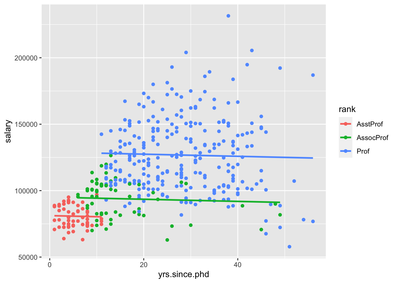
Interpret all the model coefficients by applying the techniques you learned above. These interpretations will differ from those in m1 and m2 – coefficients are defined / interpreted differently depending upon what other predictors are in the model. HINT:

• First write out the estimated model formula: \[ \widehat{salary} = 81186 - 80 \cdot yrs.since.phd + 13932 \cdot rankAssocProf + 47860 \cdot rankProf \]
• Then, notice that the presence of a categorical variable results in the separation of the model formula by group. To this end, plug in 0’s and 1’s to obtain 3 separate model formulas for the ranks: \[ \widehat{salary}_{AssistProf} = 81186 -80 \cdot yrs.since.phd. \\ \widehat{salary}_{AssocProf} = 95118 -80 \cdot yrs.since.phd. \\ \widehat{salary}_{Prof} = 1029046 -80 \cdot yrs.since.phd. \] Is there anything that strikes you as odd about this model? Do you have any concerns about the variables we are including?

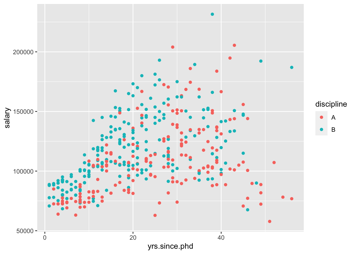
Let’s try another model with a categorical variable and a quantitative variable. This time, let’s use discipline as our categorical variable.

m4 <- lm(salary ~ yrs.since.phd + discipline, data = Salaries)
summary(m4)

## 
## Call:
## lm(formula = salary ~ yrs.since.phd + discipline, data = Salaries)
## 
## Residuals:
##    Min     1Q Median     3Q    Max 
## -79837 -16607  -4373  15679  93098 
## 
## Coefficients:
##               Estimate Std. Error t value Pr(>|t|)    
## (Intercept)    80158.3     3328.3  24.083  < 2e-16 ***
## yrs.since.phd   1118.5      105.8  10.576  < 2e-16 ***
## disciplineB    15784.2     2733.3   5.775 1.56e-08 ***
## ---
## Signif. codes:  0 '***' 0.001 '**' 0.01 '*' 0.05 '.' 0.1 ' ' 1
## 
## Residual standard error: 26470 on 394 degrees of freedom
## Multiple R-squared:  0.2401, Adjusted R-squared:  0.2362 
## F-statistic: 62.24 on 2 and 394 DF,  p-value: < 2.2e-16

Again, I’ll visualize that relationship for you,

p3 <- ggplot(
  Salaries,
  aes(x = yrs.since.phd, y = salary, color = discipline)
) +
  geom_point()
p3

p3 + moderndive::geom_parallel_slopes(se = FALSE)

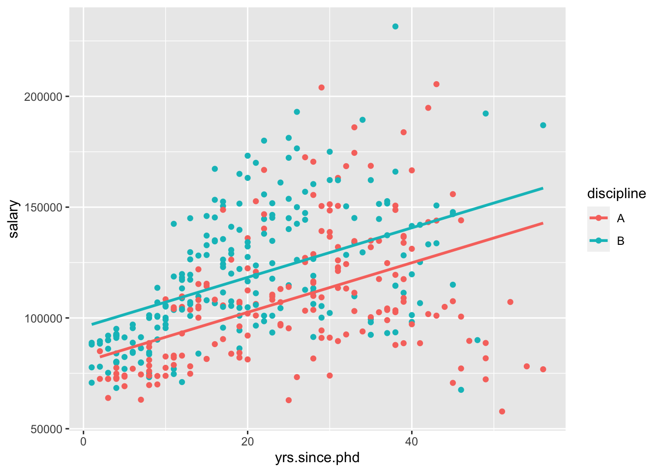
• “For a 1-year increase in years since PhD, we would expect a 1118-dollar increase in salary, holding the discipline constant.”

• “Compared to discipline A, we would expect people in discipline B to be making 15784 dollars more, holding years of experience constant.”

This model assumes that the relationship between yrs.since.phd and salary is the same between disciplines. However, we could include an interaction between the two variables,

m5 <- lm(salary~yrs.since.phd+discipline+yrs.since.phd*discipline, data = Salaries)
summary(m5)

## 
## Call:
## lm(formula = salary ~ yrs.since.phd + discipline + yrs.since.phd * 
##     discipline, data = Salaries)
## 
## Residuals:
##    Min     1Q Median     3Q    Max 
## -84580 -16974  -3620  15733  92072 
## 
## Coefficients:
##                           Estimate Std. Error t value Pr(>|t|)    
## (Intercept)                84845.4     4283.9  19.806  < 2e-16 ***
## yrs.since.phd                933.9      150.0   6.225 1.24e-09 ***
## disciplineB                 7530.0     5492.2   1.371   0.1711    
## yrs.since.phd:disciplineB    365.3      211.0   1.731   0.0842 .  
## ---
## Signif. codes:  0 '***' 0.001 '**' 0.01 '*' 0.05 '.' 0.1 ' ' 1
## 
## Residual standard error: 26400 on 393 degrees of freedom
## Multiple R-squared:  0.2458, Adjusted R-squared:  0.2401 
## F-statistic:  42.7 on 3 and 393 DF,  p-value: < 2.2e-16

Now, we can visualize this using standard ggplot2 geom_s,

p3 + geom_smooth(method = "lm", se = FALSE)

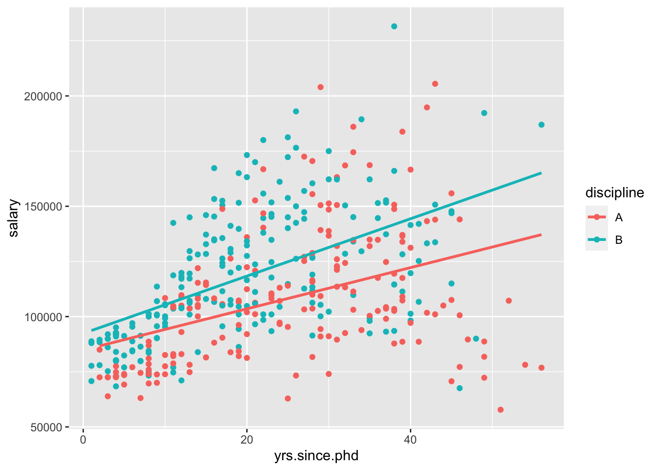
\[ \widehat{salary}_{A} = 84845 + 934\cdot yrs.since.phd \\ \widehat{salary}_{B} = 84845 + 934\cdot yrs.since.phd + 7530 + 365\cdot yrs.since.phd \\ \widehat{salary}_{B} = (84845+ 7530) + (934 + 365)\cdot yrs.since.phd \\ \widehat{salary}_{B} = 92375 + 1299\cdot yrs.since.phd \]

Which of those two models do you prefer?

8.5.1 Models with 2 quantitative predictors

Let’s include both yrs.since.phd and yrs.service in one model.

m6 <- lm(salary~yrs.since.phd+yrs.service, data=Salaries)
summary(m6)

## 
## Call:
## lm(formula = salary ~ yrs.since.phd + yrs.service, data = Salaries)
## 
## Residuals:
##    Min     1Q Median     3Q    Max 
## -79735 -19823  -2617  15149 106149 
## 
## Coefficients:
##               Estimate Std. Error t value Pr(>|t|)    
## (Intercept)    89912.2     2843.6  31.620  < 2e-16 ***
## yrs.since.phd   1562.9      256.8   6.086 2.75e-09 ***
## yrs.service     -629.1      254.5  -2.472   0.0138 *  
## ---
## Signif. codes:  0 '***' 0.001 '**' 0.01 '*' 0.05 '.' 0.1 ' ' 1
## 
## Residual standard error: 27360 on 394 degrees of freedom
## Multiple R-squared:  0.1883, Adjusted R-squared:  0.1842 
## F-statistic: 45.71 on 2 and 394 DF,  p-value: < 2.2e-16

If we were going to visualize this model, what would it look like?

Interpret the yrs.service coefficient.

“For a 1-year increase in years of service, we would expect a $629 decrease in salary, holding years since PhD constant.”

8.5.2 Models with 2 categorical predictors

We could fit a model with rank and sex as our two predictors,

m7 <- lm(salary ~ rank + sex, data = Salaries)

8.5.3 Lots of variables

You don’t have to be limited to just two variables! Multiple regression models can contain as many variables as you (as the analyst) find appropriate.

m8 <- lm(salary ~ yrs.since.phd + yrs.service + rank + discipline + sex + yrs.service*discipline, data = Salaries)
summary(m8)

## 
## Call:
## lm(formula = salary ~ yrs.since.phd + yrs.service + rank + discipline + 
##     sex + yrs.service * discipline, data = Salaries)
## 
## Residuals:
##    Min     1Q Median     3Q    Max 
## -71931 -13185  -1896  10086  94613 
## 
## Coefficients:
##                         Estimate Std. Error t value Pr(>|t|)    
## (Intercept)              70095.1     4885.5  14.348  < 2e-16 ***
## yrs.since.phd              554.0      239.7   2.311  0.02136 *  
## yrs.service               -687.7      226.7  -3.033  0.00258 ** 
## rankAssocProf            12166.2     4132.9   2.944  0.00344 ** 
## rankProf                 43744.8     4249.5  10.294  < 2e-16 ***
## disciplineB               6990.5     3907.6   1.789  0.07440 .  
## sexMale                   5223.0     3840.6   1.360  0.17463    
## yrs.service:disciplineB    420.0      177.4   2.367  0.01841 *  
## ---
## Signif. codes:  0 '***' 0.001 '**' 0.01 '*' 0.05 '.' 0.1 ' ' 1
## 
## Residual standard error: 22410 on 389 degrees of freedom
## Multiple R-squared:  0.4624, Adjusted R-squared:  0.4527 
## F-statistic:  47.8 on 7 and 389 DF,  p-value: < 2.2e-16

8.6 Homework

Before we meet next time, I’d like you to try some visualization and modeling on your own.

• Start a new RMarkdown document
• Load the following packages at the top of your Rmd: dplyr, ggplot2, fivethirtyeight, skimr
• When interpreting visualizations, models, etc, be sure to do so in a contextually meaningful way.
• This homework is a resource for you. Record all work that is useful for your current learning & future reference. Further, try your best, but don’t stay up all night trying to finish all of the exercises! We’ll discuss any questions / material you didn’t get to tomorrow.

For this assignment, you will need an additional package I forgot to tell you to install before! So, run the following code in your Console:

install.packages("palmerpenguins")

## 
## The downloaded binary packages are in
##  /var/folders/m7/f7bf48x11fdgvv8wy155qyyhhxrxdr/T//RtmpAbQysS/downloaded_packages

Do not include this code in your RMarkdown document, otherwise you will re-download the package every time you knit!

Once the package has downloaded, you can load the package and load the data

library(palmerpenguins)
data(penguins)

Horst, Hill, and Gorman (2020)

You should read about the data in the documentation,

?penguins

Let response variable \(Y\) be the length in mm of a penguin’s flipper and \(X\) be their body mass in grams. Then the (population) linear regression model of \(Y\) vs \(X\)

is

\[ Y=\beta_0+\beta_1\cdot X+ \epsilon \]

Note that the \(\beta_i\) represent the population coefficients. We can’t measure all penguins, thus don’t know the “true” values of the \(\beta_i\). Rather, we can use sample data to estimate the\(\beta_i\) by \(\hat{\beta}_i\).

That is, the sample estimate of the population model trend is

\[ Y=\hat{\beta}_0+\hat{\beta}_1\cdot X \] In choosing the “best” estimates \(\hat{\beta}_i\), we’re looking for the coefficients that best describe the relationship between \(Y\) and \(X\) among the sample subjects. In the visual below, we can see that the red line does a better job at capturing this relationship than the blue line does:

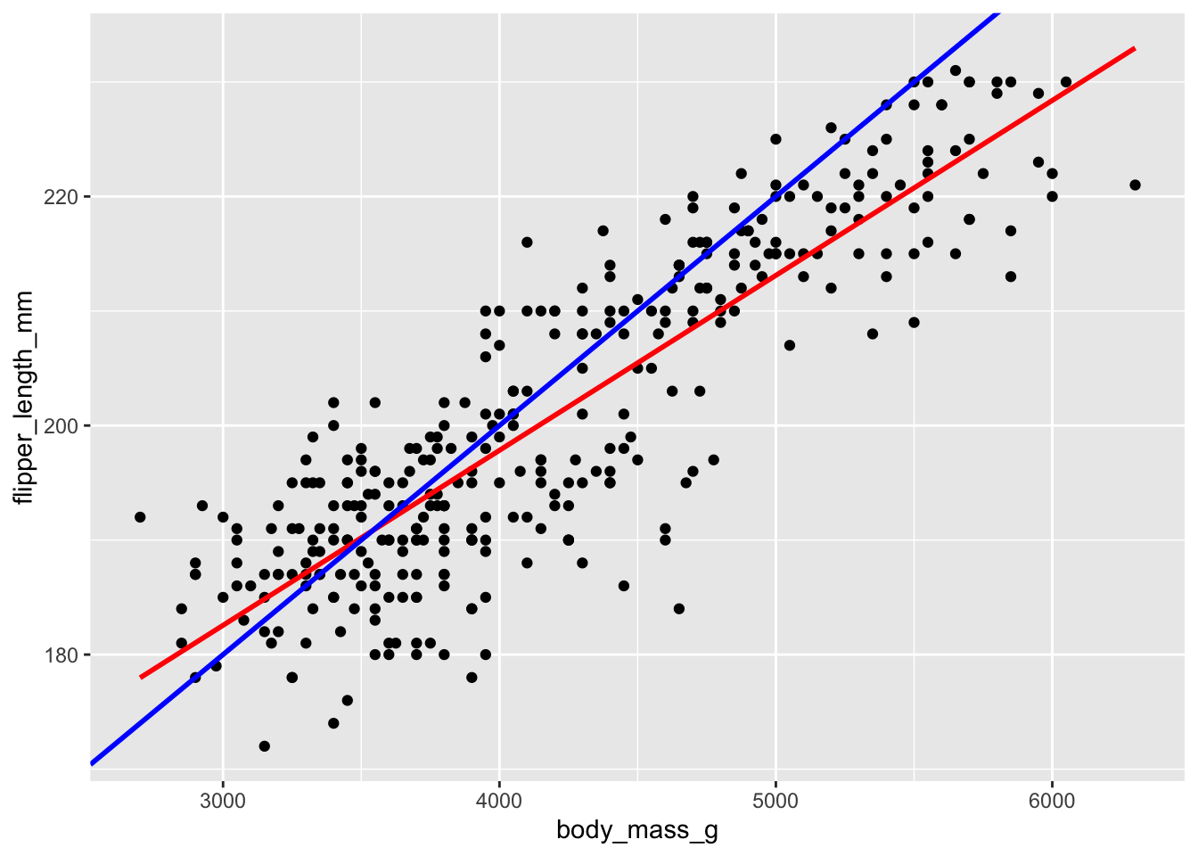
Mainly, on average, the individual points fall closer to the red line than the blue line. The distance between an individual observation and its model value (prediction) is called a residual.

\[ \epsilon_i = y_i - \hat{y}_i \] Let’s use our sample data to estimate the population model.

1. Fit a simple linear regression, and look at the summary:

penguinmod <- lm(flipper_length_mm~body_mass_g, data=penguins)
summary(penguinmod)

## 
## Call:
## lm(formula = flipper_length_mm ~ body_mass_g, data = penguins)
## 
## Residuals:
##      Min       1Q   Median       3Q      Max 
## -23.7626  -4.9138   0.9891   5.1166  16.6392 
## 
## Coefficients:
##              Estimate Std. Error t value Pr(>|t|)    
## (Intercept) 1.367e+02  1.997e+00   68.47   <2e-16 ***
## body_mass_g 1.528e-02  4.668e-04   32.72   <2e-16 ***
## ---
## Signif. codes:  0 '***' 0.001 '**' 0.01 '*' 0.05 '.' 0.1 ' ' 1
## 
## Residual standard error: 6.913 on 340 degrees of freedom
##   (2 observations deleted due to missingness)
## Multiple R-squared:  0.759,  Adjusted R-squared:  0.7583 
## F-statistic:  1071 on 1 and 340 DF,  p-value: < 2.2e-16

2. What is the equation of the fitted model?

3. Interpret the slope and the intercept.

4. Make predictions for the flipper length of the following two penguins:

## # A tibble: 2 x 4
##   species island    flipper_length_mm body_mass_g
##   <fct>   <fct>                 <int>       <int>
## 1 Adelie  Torgersen               181        3750
## 2 Gentoo  Biscoe                  210        4200

5. What are the residuals for these two penguins?

6. penguin_mod is an lm “object.” Not only does it contain info about the model coefficients, it contains the numerical values of the residuals (residuals) and model predictions (fitted.values) for each penguin in the data set:

class(penguinmod)

## [1] "lm"

names(penguinmod)

##  [1] "coefficients"  "residuals"     "effects"       "rank"         
##  [5] "fitted.values" "assign"        "qr"            "df.residual"  
##  [9] "na.action"     "xlevels"       "call"          "terms"        
## [13] "model"

You can print out all the residuals in the data frame by doing something like,

residuals(penguinmod)

##            1            2            3            5            6            7 
## -13.01424280  -8.77803858   8.62371500   3.56853188  -2.48665124 -11.10475335 
##            8            9           10           11           12           13 
## -13.14446474   3.18663399 -11.65220061  -1.14008078 -13.25044702  -3.61248922 
##           14           15           16           17           18           19 
##  -3.77803858  -5.94358795  -8.25044702   5.56853188  -8.47117951  -3.52197867 
##           20           21           22           23           24           25 
##  -6.88840483 -14.66767234 -11.72285546  -5.77803858 -12.06942592 -14.77803858 
##           26           27           28           29           30           31 
##  -7.77803858  -7.95905968   1.38751078 -12.84869344 -17.06942592  -8.37628500 
##           32           33           34           35           36           37 
## -18.30563014   0.85991922 -12.30563014   7.47802133  -4.12460905  -7.06942592 
##           38           39           40           41           42           43 
## -10.95905968  -6.14008078 -23.76256685  -2.84869344  -1.30563014   1.91510234 
##           44           45           46           47           48           49 
##  -7.94358795   2.44269390 -16.99877107  -7.04957023  -3.17540821   0.56853188 
##           50           51           52           53           54           55 
##  -9.12460905  -4.19526390 -14.41599639   0.56853188   1.40298251   5.97028546 
##           56           57           58           59           60           61 
##  -2.25044702  -4.95905968  -1.77803858   0.73408124  -0.01424280   0.15130656 
##           62           63           64           65           66           67 
##  -8.94358795  -6.72285546  -6.59701749   3.73408124  -5.06942592   7.09612344 
##           68           69           70           71           72           73 
## -11.36081327   6.67889812  -6.70738373  -1.72285546  -6.30563014   5.04094032 
##           74           75           76           77           78           79 
##  -3.12460905  -3.25044702  -6.65220061  -2.25044702 -12.30563014  -3.95905968 
##           80           81           82           83           84           85 
##  -2.83322170   3.38751078 -12.52636263  -7.77803858  -7.88840483   3.09612344 
##           86           87           88           89           90           91 
##   3.04094032  -4.77803858  -1.19526390  -8.06942592  -1.72285546  11.04094032 
##           92           93           94           95           96           97 
##   2.58400361  -3.66767234 -18.70738373  -0.14008078   5.58400361  -3.25044702 
##           98           99          100          101          102          103 
##  -7.17979217  -3.02971454  -7.36081327  -1.63234491  -5.90826052  -0.70299977 
##          104          105          106          107          108          109 
## -11.65220061  11.58838757  -6.95905968   4.98575720  -6.30563014  -4.23059133 
##          110          111          112          113          114          115 
## -12.67205630   2.84006353 -15.99877107   7.38751078  -5.03409850  -5.30563014 
##          116          117          118          119          120          121 
##  -2.97891538   6.97028546   4.60385931   1.09612344   1.47802133   2.15130656 
##          122          123          124          125          126          127 
##   7.80473610 -13.43146812   6.07626775   2.67889812   1.16677830   4.24181711 
##          128          129          130          131          132          133 
##  -7.41599639   7.67889812  12.16677830   2.47802133   6.80473610   2.80473610 
##          134          135          136          137          138          139 
##  -6.08928162  -2.04957023  -6.30563014   5.76940867   2.54867619  -3.66767234 
##          140          141          142          143          144          145 
##  -8.65220061   4.33232766  -2.81336601   4.67889812  -3.63234491   9.44269390 
##          146          147          148          149          150          151 
##  -7.48665124 -11.65220061  -5.81336601   5.56853188  -1.01424280  -6.25044702 
##          152          153          154          155          156          157 
##   3.16677830   5.52882049   6.19772176   5.29261627  -5.80227824  -4.21950356 
##          158          159          160          161          162          163 
##   3.76502471   0.94604581   2.83567957   5.05641205  -0.40052465   6.23743315 
##          164          165          166          167          168          169 
##  -5.51089090   6.23743315 -13.09366558   9.11159517  -9.09366558   9.87539095 
##          170          171          172          173          174          175 
## -11.96782760  -1.05395419   3.54429222  -5.80227824   1.89086269   9.05641205 
##          176          177          178          179          180          181 
##   1.12706691   1.89086269   0.36327113  16.63918673  -8.03848246   3.00122893 
##          182          183          184          185          186          187 
##  -1.51089090   5.07188379   0.47363737  -6.87293309   0.85115130   4.59947535 
##          188          189          190          191          192          193 
##   0.78049644   0.65465847   2.07188379   4.82020783 -10.45570778  10.93057408 
##          194          195          196          197          198          199 
##   1.19772176   7.58400361   6.70984159   0.48910910   5.41845425   9.11159517 
##          200          201          202          203          204          205 
##   5.78049644  -1.63672887  -2.69191200  -0.81774997   2.30808800   6.05641205 
##          206          207          208          209          210          211 
##  11.89086269   5.41845425   6.12706691   5.58400361   6.89086269   3.29261627 
##          212          213          214          215          216          217 
##   2.48910910   7.11159517   3.30808800  10.05641205   7.96151754  10.47363737 
##          218          219          220          221          222          223 
##   6.19772176   6.23743315   3.67013020  11.47363737   1.48910910   6.70984159 
##          224          225          226          227          228          229 
##   7.89086269   6.36327113   0.83567957   7.47363737   4.67013020   2.00122893 
##          230          231          232          233          234          235 
##  -8.38505292   5.70984159  -4.62125714   4.61933104   1.01670066   3.09173948 
##          236          237          238          239          240          241 
##   5.54429222   2.70984159   5.72531332  11.00122893   0.30808800   0.80035214 
##          242          243          244          245          246          247 
##   8.48910910   5.65465847   8.78049644   2.70984159   0.96151754   3.18225003 
##          248          249          250          251          252          253 
##   9.83567957   4.03655636  10.80035214  -4.38066896   8.07188379   8.18225003 
##          254          255          256          257          258          259 
##   5.72531332   2.27276058   7.25290488   7.09173948  -5.74709512   1.47363737 
##          260          261          262          263          264          265 
##  -1.74709512   1.38312682 -11.74709512   2.89086269   1.37874286   5.23743315 
##          266          267          268          269          270          271 
##   9.25290488  13.43830994   3.90633442   5.80035214  -6.38505292   2.03655636 
##          273          274          275          276          277          278 
##   4.18225003  -2.56607402  -4.16432043  -6.21950356   1.80473610  -0.30563014 
##          279          280          281          282          283          284 
##   0.51334876  -2.57716179   3.36765509   0.93057408  -8.37628500   2.98575720 
##          285          286          287          288          289          290 
##  -5.12460905   4.74955298  -1.77803858  -0.39614069  -8.25044702   2.40298251 
##          291          292          293          294          295          296 
##  -1.34095757   2.40298251   9.85991922 -12.25044702   0.56853188  -8.94358795 
##          297          298          299          300          301          302 
## -10.72285546   2.33232766   5.97028546  -1.77803858   7.85991922  -3.12460905 
##          303          304          305          306          307          308 
##  11.33232766   5.22196142  -2.25044702  -1.23497529   1.38751078  -1.41599639 
##          309          310          311          312          313          314 
##  -0.90387656   3.63918673   3.27714454   2.69436986  -0.54183436  -0.05395419 
##          315          316          317          318          319          320 
##  14.02546859  -0.47117951  12.93057408  -5.48665124   5.04094032   5.80473610 
##          321          322          323          324          325          326 
##   3.13145087  -3.70738373   1.33232766   9.58400361   0.62371500   5.13145087 
##          327          328          329          330          331          332 
##  11.47802133   3.93057408   1.27714454   4.40298251  -0.90387656   7.56853188 
##          333          334          335          336          337          338 
##   4.62371500   4.40298251   7.22196142   3.42283821   8.93057408  -3.48665124 
##          339          340          341          342          343          344 
##   2.51334876   9.16677830  13.33232766  -1.39614069  10.63918673   3.60385931

7. See if you can confirm that the mean residual equals 0. This property always holds for regression models!

summary(residuals(penguinmod))

##     Min.  1st Qu.   Median     Mean  3rd Qu.     Max. 
## -23.7626  -4.9138   0.9891   0.0000   5.1166  16.6392

mean(residuals(penguinmod))

## [1] -4.416659e-16

8. Calculate the standard deviation of the residuals. Where does this information appear in summary(penguinmod) (within rounding error)? SIDENOTE: The Residual standard error is calculated slightly differently than the standard deviation of residuals. Let \(\epsilon_i\) denote a residual for case \(i\), \(n\) as sample size, and \(k\) the number of coefficients in our model (here we have 2), then the standard deviation of residuals are

\[ \frac{\sum_{i=1}^n \epsilon_i^2}{n-1} \] whereas the residual standard error is

\[ \frac{\sum_{i=1}^n \epsilon_i^2}{n-k} \]

sd(residuals(penguinmod))

## [1] 6.903249

Now that you have thought a lot about a simple linear regression model, explore some more variables. Try making plots to see if you can find other variables that help explain some variability in flipper_length_mm.

Then, try out a variety of models. Try using more than one variable, making parallel slopes, including interaction effects, etc. You can name your models as you go, but I am most interested in your “final” favorite model.

9. Write down your favorite model,

favmod <- lm(flipper_length_mm ~ species + bill_depth_mm + body_mass_g + sex, 
             data = penguins)
summary(favmod)

## 
## Call:
## lm(formula = flipper_length_mm ~ species + bill_depth_mm + body_mass_g + 
##     sex, data = penguins)
## 
## Residuals:
##     Min      1Q  Median      3Q     Max 
## -14.358  -3.185   0.009   3.036  17.782 
## 
## Coefficients:
##                   Estimate Std. Error t value Pr(>|t|)    
## (Intercept)      1.497e+02  6.372e+00  23.494  < 2e-16 ***
## speciesChinstrap 5.491e+00  7.781e-01   7.057 1.02e-11 ***
## speciesGentoo    2.227e+01  2.131e+00  10.453  < 2e-16 ***
## bill_depth_mm    9.786e-01  3.639e-01   2.689  0.00753 ** 
## body_mass_g      5.859e-03  9.572e-04   6.121 2.66e-09 ***
## sexmale          1.466e+00  9.259e-01   1.584  0.11426    
## ---
## Signif. codes:  0 '***' 0.001 '**' 0.01 '*' 0.05 '.' 0.1 ' ' 1
## 
## Residual standard error: 5.295 on 327 degrees of freedom
##   (11 observations deleted due to missingness)
## Multiple R-squared:  0.8594, Adjusted R-squared:  0.8573 
## F-statistic: 399.8 on 5 and 327 DF,  p-value: < 2.2e-16

10. Why is this your preferred model? What is good about it?

11. How would you visualize your model object?

ggplot(penguins, aes(x=body_mass_g, y=flipper_length_mm, color = species)) + 
  geom_point()

## Warning: Removed 2 rows containing missing values (geom_point).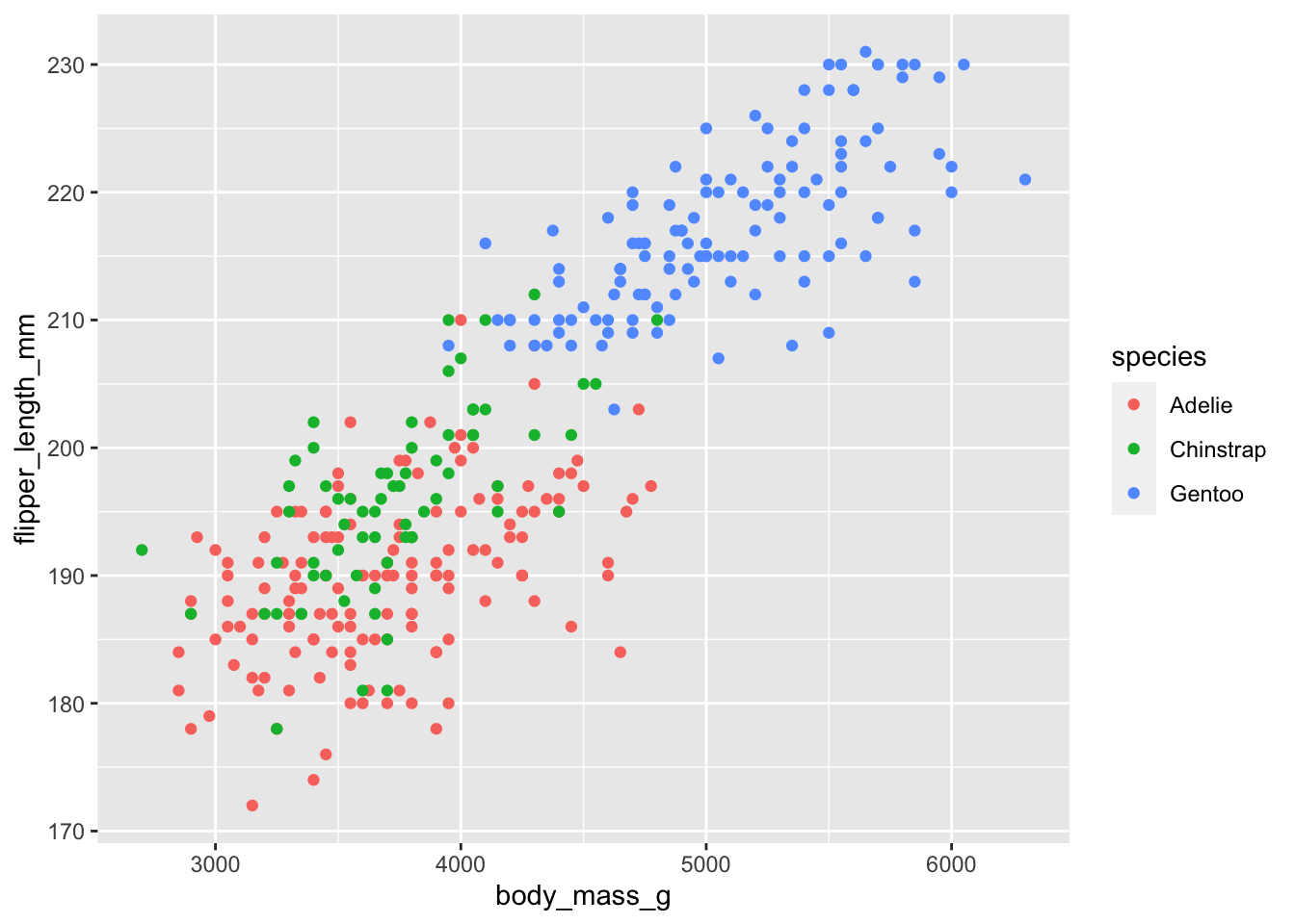

References

Horst, Allison Marie, Alison Presmanes Hill, and Kristen B Gorman. 2020. Palmerpenguins: Palmer Archipelago (Antarctica) Penguin Data. https://doi.org/10.5281/zenodo.3960218.

Wickham, Hadley, and Garrett Grolemund. 2017. R for Data Science. O’Reilly. https://r4ds.had.co.nz.