Chapter 9 Data wrangling for model assessment
[This “chapter” is essentially the same as 3, but with some of the notes I wrote in the document as we went.]
We’ll talk about the dplyr package, and assessing models.
Much of this code was adapted from Master the Tidyverse
9.1 dplyr verbs
We have already seen some dplyr verbs, but we are going to need more as we move on. So, let’s spend some time focusing on them. Here are the main verbs we will cover:
| verb | action | example |
|---|---|---|
select() |
take a subset of columns | select(x,y), select(-x) |
filter() |
take a subset of rows | filter(x == __, y > __) |
arrange() |
reorder the rows | arrange(x), arrange(desc(x)) |
summarize() |
a many-to-one or many-to-few summary | summarize(mean(x), median(y)) |
group_by() |
group the rows by a specified column | group_by(x) %>% something() |
mutate() |
a many-to-many operation that creates a new variable | mutate(x = ___, y = ___) |
We’ll use the babynames package to play with the verbs, so let’s begin by loading that dataset.
We could skim the data, to learn something about it:
| Name | babynames |
| Number of rows | 1924665 |
| Number of columns | 5 |
| _______________________ | |
| Column type frequency: | |
| character | 2 |
| numeric | 3 |
| ________________________ | |
| Group variables | None |
Variable type: character
| skim_variable | n_missing | complete_rate | min | max | empty | n_unique | whitespace |
|---|---|---|---|---|---|---|---|
| sex | 0 | 1 | 1 | 1 | 0 | 2 | 0 |
| name | 0 | 1 | 2 | 15 | 0 | 97310 | 0 |
Variable type: numeric
| skim_variable | n_missing | complete_rate | mean | sd | p0 | p25 | p50 | p75 | p100 | hist |
|---|---|---|---|---|---|---|---|---|---|---|
| year | 0 | 1 | 1974.85 | 34.03 | 1880 | 1951 | 1985 | 2003 | 2017.00 | ▁▂▃▅▇ |
| n | 0 | 1 | 180.87 | 1533.34 | 5 | 7 | 12 | 32 | 99686.00 | ▇▁▁▁▁ |
| prop | 0 | 1 | 0.00 | 0.00 | 0 | 0 | 0 | 0 | 0.08 | ▇▁▁▁▁ |
9.1.1 select()
## # A tibble: 1,924,665 x 2
##    name        prop
##    <chr>      <dbl>
##  1 Mary      0.0724
##  2 Anna      0.0267
##  3 Emma      0.0205
##  4 Elizabeth 0.0199
##  5 Minnie    0.0179
##  6 Margaret  0.0162
##  7 Ida       0.0151
##  8 Alice     0.0145
##  9 Bertha    0.0135
## 10 Sarah     0.0132
## # … with 1,924,655 more rows- Alter the code to select just the
ncolumn
## # A tibble: 1,924,665 x 1
##        n
##    <int>
##  1  7065
##  2  2604
##  3  2003
##  4  1939
##  5  1746
##  6  1578
##  7  1472
##  8  1414
##  9  1320
## 10  1288
## # … with 1,924,655 more rows
9.1.1.1 select() helpers
:select range of columns,select(storms, storm:pressure)-select every column butselect(storms, -c(storm, pressure))starts_with()select columns that start with…select(storms, starts_with("w"))ends_with()select columns that end with…select(storms, ends_with("e"))- …and more! Check out the Data Transformation cheatsheet
9.1.2 filter()
extract rows that meet logical criteria
## # A tibble: 169 x 5
##     year sex   name       n    prop
##    <dbl> <chr> <chr>  <int>   <dbl>
##  1  1880 F     Amelia   221 0.00226
##  2  1881 F     Amelia   235 0.00238
##  3  1882 F     Amelia   252 0.00218
##  4  1883 F     Amelia   262 0.00218
##  5  1884 F     Amelia   315 0.00229
##  6  1885 F     Amelia   298 0.00210
##  7  1886 F     Amelia   326 0.00212
##  8  1887 F     Amelia   344 0.00221
##  9  1888 F     Amelia   358 0.00189
## 10  1889 F     Amelia   346 0.00183
## # … with 159 more rows
Notice I’m using ==, which tests if things are equal. In R, = sets something. There are other logical comparisons you can use
| x < y | less than |
| x > y | greater than |
| x == y | equal to |
| x <= y | less than or equal to |
| x >= y | greater than or equal to |
| x != y | not equal to |
| x %in% y | group membership |
| is.na(x) | is NA |
| !is.na(x) | is not NA |
- Now, see if you can use the logical operators to manipulate our code to show:
- All of the names where
propis greater than or equal to 0.08 - All of the children named “Sea”
- All of the names that have a missing value for
n(Hint: this should return an empty data set).
Common mistakes:
- using
=instead of== - forgetting quotes
We can also filter rows that match every logical criteria,
## # A tibble: 1 x 5
##    year sex   name       n    prop
##   <dbl> <chr> <chr>  <int>   <dbl>
## 1  1880 F     Amelia   221 0.00226
For this, you need to use Boolean operators
| a & b | and |
| a | b | or |
| xor(a, b) | exactly or |
| !a | not |
| a %in% c(a, b) | one of (in) |
- Use Boolean operators to alter the code below to return only the rows that contain:
- Girls named Sea
- Names that were used by exactly 5 or 6 children in 1880
- Names that are one of Acura, Lexus, or Yugo
## # A tibble: 57 x 5
##     year sex   name      n       prop
##    <dbl> <chr> <chr> <int>      <dbl>
##  1  1990 F     Lexus    36 0.0000175
##  2  1990 M     Lexus    12 0.00000558
##  3  1991 F     Lexus   102 0.0000502
##  4  1991 M     Lexus    16 0.00000755
##  5  1992 F     Lexus   193 0.0000963
##  6  1992 M     Lexus    25 0.0000119
##  7  1993 F     Lexus   285 0.000145
##  8  1993 M     Lexus    30 0.0000145
##  9  1994 F     Lexus   381 0.000195
## 10  1994 F     Acura     6 0.00000308
## # … with 47 more rows9.1.3 arrange()
Orders rows from smallest to largest values
- Arrange babynames by n. Add prop as a second (tie breaking) variable to arrange by.
## # A tibble: 1,924,665 x 5
##     year sex   name          n      prop
##    <dbl> <chr> <chr>     <int>     <dbl>
##  1  1880 F     Adelle        5 0.0000512
##  2  1880 F     Adina         5 0.0000512
##  3  1880 F     Adrienne      5 0.0000512
##  4  1880 F     Albertine     5 0.0000512
##  5  1880 F     Alys          5 0.0000512
##  6  1880 F     Ana           5 0.0000512
##  7  1880 F     Araminta      5 0.0000512
##  8  1880 F     Arthur        5 0.0000512
##  9  1880 F     Birtha        5 0.0000512
## 10  1880 F     Bulah         5 0.0000512
## # … with 1,924,655 more rows- Can you tell what the smallest value of
nis? Any guesses why?
Another helpful function is desc(), which changes the ordering to largest smallest,
## # A tibble: 1,924,665 x 5
##     year sex   name        n   prop
##    <dbl> <chr> <chr>   <int>  <dbl>
##  1  1947 F     Linda   99686 0.0548
##  2  1948 F     Linda   96209 0.0552
##  3  1947 M     James   94756 0.0510
##  4  1957 M     Michael 92695 0.0424
##  5  1947 M     Robert  91642 0.0493
##  6  1949 F     Linda   91016 0.0518
##  7  1956 M     Michael 90620 0.0423
##  8  1958 M     Michael 90520 0.0420
##  9  1948 M     James   88588 0.0497
## 10  1954 M     Michael 88514 0.0428
## # … with 1,924,655 more rows- Use
desc()to find the names with the highestprop.
## # A tibble: 1,924,665 x 5
##     year sex   name        n   prop
##    <dbl> <chr> <chr>   <int>  <dbl>
##  1  1880 M     John     9655 0.0815
##  2  1881 M     John     8769 0.0810
##  3  1880 M     William  9532 0.0805
##  4  1883 M     John     8894 0.0791
##  5  1881 M     William  8524 0.0787
##  6  1882 M     John     9557 0.0783
##  7  1884 M     John     9388 0.0765
##  8  1882 M     William  9298 0.0762
##  9  1886 M     John     9026 0.0758
## 10  1885 M     John     8756 0.0755
## # … with 1,924,655 more rows- Use
desc()to find the names with the highestn.
9.2 %>%, the pipe
I %>%
— Hadley Wickham (@hadleywickham) February 11, 2021
tumble(out_of = "bed") %>%
stumble(to = "the kitchen") %>%
pour(who = "myself", unit = "cup", what = "ambition") %>%
yawn() %>%
stretch() %>%
try(come_to_live()) https://t.co/plnA2dZdJ4
In other words, you can nest functions together in R, much like
\[ f(g(x)) \]
but, once you go beyond a function or two, that becomes hard to read.
try(come_to_life(stretch(yawn(pour(stumble(tumble(I, out_of = "bed"), to = "the kitchen"), who = "myself", unit = "cup", what = "ambition")))))The pipe allows you to unnest your functions, and pass data along a pipeline.
I %>%
  tumble(out_of = "bed") %>%
  stumble(to = "the kitchen") %>%
  pour(who = "myself", unit = "cup", what = "ambition") %>%
  yawn() %>%
  stretch() %>%
  try(come_to_life())
(Those examples are not valid R code!)
We could see this with a more real-life example:
## # A tibble: 14,024 x 2
##    name          n
##    <chr>     <int>
##  1 Noah      19613
##  2 Liam      18355
##  3 Mason     16610
##  4 Jacob     15938
##  5 William   15889
##  6 Ethan     15069
##  7 James     14799
##  8 Alexander 14531
##  9 Michael   14413
## 10 Benjamin  13692
## # … with 14,014 more rows
What does this code do?
## # A tibble: 14,024 x 2
##    name          n
##    <chr>     <int>
##  1 Noah      19613
##  2 Liam      18355
##  3 Mason     16610
##  4 Jacob     15938
##  5 William   15889
##  6 Ethan     15069
##  7 James     14799
##  8 Alexander 14531
##  9 Michael   14413
## 10 Benjamin  13692
## # … with 14,014 more rowsWhat does this code do?
babynames %>%
  filter(year == 2015, sex == "M") %>%
  arrange(desc(n)) %>%
  lm(prop~year, data = .) # . passes data in a different spot
##
## Call:
## lm(formula = prop ~ year, data = .)
##
## Coefficients:
## (Intercept) year
## 6.681e-05 NAWe pronounce the pipe, %>%, as “then.”
[Side note: many languages use | as the pipe, but that means “or” or “given” in R, depending on the syntax.]
- Use
%>%to write a sequence of functions that
- Filter babynames to just the girls that were born in 2015
- Select the
nameandncolumns - Arrange the results so that the most popular names are near the top.
library(ggplot2)
babynames %>%
  filter(name %in% c("Amelia", "Richard", "Sofia")) %>%
  ggplot(aes(x=year, y=n, color = name)) +
  geom_line() +
  facet_wrap(~sex)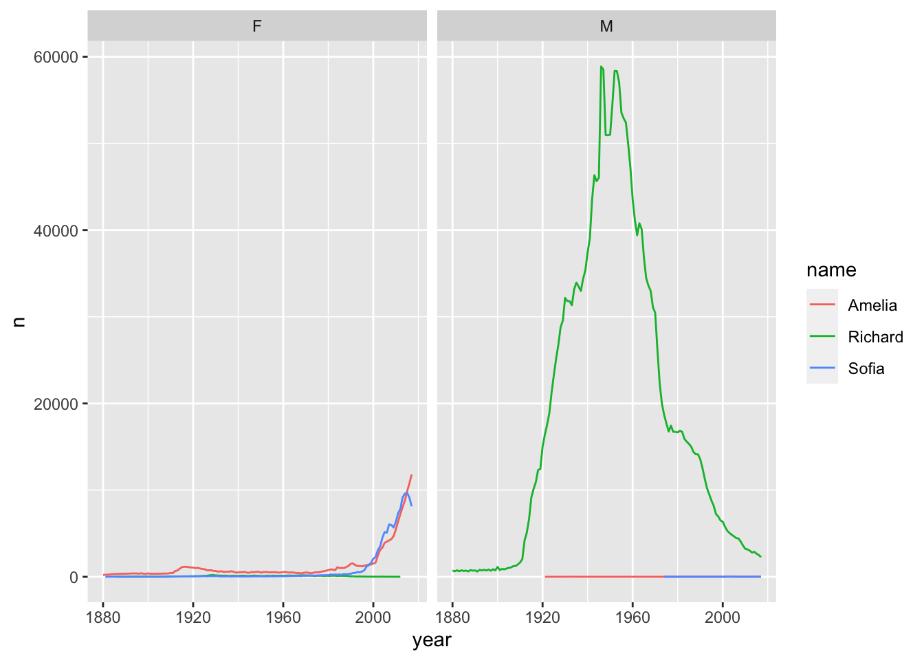
- [Combining
dplyrknowledge withggplot2!]
- Trim
babynamesto just the rows that contain a particular name and sex. This could be your name/sex or that of a friend or famous person. - Trim the result to just the columns that you’ll need for the plot
- Plot the results as a line graph with
yearon the x axis andpropon the y axis
[Hint: “trim” here is a colloquial word, you will need to translate it to the appropriate dplyr verb in each case.]
9.3 Modeling conditions
9.3.1 Least squares
When R finds the line of best fit, it is minimizing the sum of the squared residuals,
\[ SSE = \sum_{i=1}^n (y_i - \hat{y_i})^2 \] in order for the model to be appropriate, a number of conditions must be met.
- Linearity
- Independence
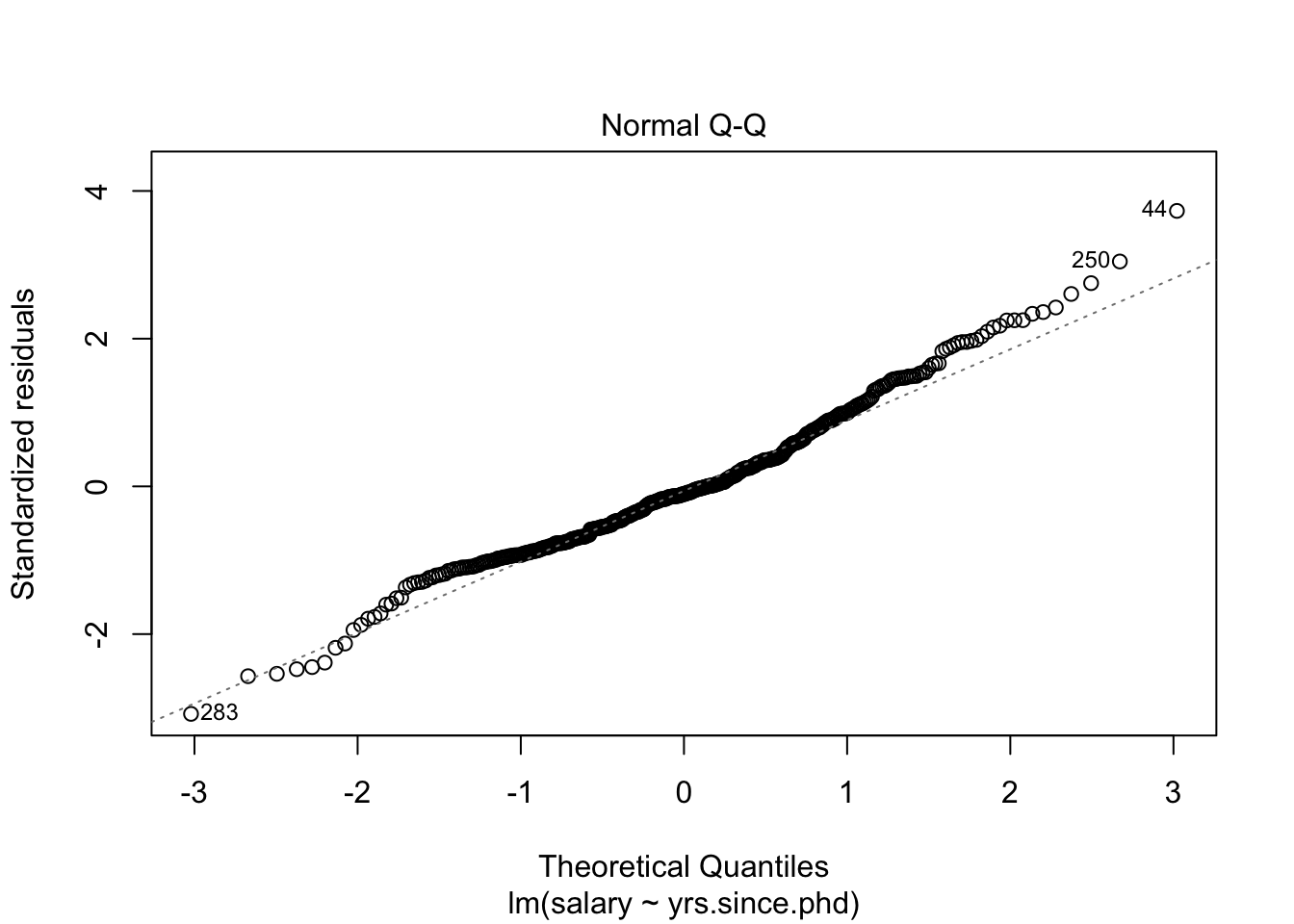
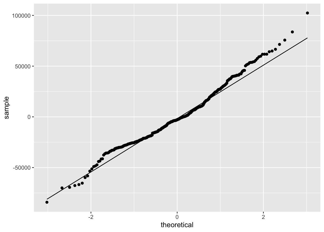
- Normality
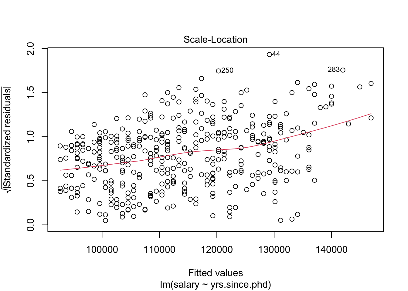
- Equality of variance
These conditions are mainly related to the distribution of the residuals.
| Assumption | Consequence | Diagnostic | Solution |
|---|
Independence | inaccurate inference | common sense/context | use a different technique/ don’t model \(E(\epsilon)=0\) | lack of model fit | plot of residuals vs. fitted values | transform \(x\) and/or \(y\) \(Var(\epsilon)=\sigma^2\) | inaccurate inference | plot of residuals v. fitted values | transform \(y\) \(\epsilon\sim N(\mu, \sigma)\) | if extreme, inaccurate inference | QQ plot | transform \(y\)
We would like to be able to work with the residuals from our models to assess whether the conditions are met, as well as to determine which model explains the most variability.
We would like to be able to work with the model objects we created yesterday using dplyr verbs, but model objects are untidy objects. This is where the broom package comes in! broom helps you tidy up your models. Its two most useful functions are augment and tidy.
Let’s re-create our simple linear regression model from before (again, I’m hoping this isn’t just hanging out in your Environment already!).
Let’s augment() that model.
Look at the new object in your environment. What is it like?
One parameter to augment() is data=. Let’s try again with that,
What’s different about that object?
We could use this augmented version of our dataset to do things like look for the largest residuals.
- Use a
dplyrverb to find the rows where we over-predicted the most.
## # A tibble: 397 x 12
##    rank  discipline yrs.since.phd yrs.service sex   salary .fitted  .resid
##    <fct> <fct>              <int>       <int> <fct>  <int>   <dbl>   <dbl>
##  1 Prof  B                     38          38 Male  231545 129162. 102383.
##  2 Prof  A                     51          51 Male   57800 141971. -84171.
##  3 Prof  A                     29           7 Male  204000 120294.  83706.
##  4 Prof  B                     26          19 Male  193000 117338.  75662.
##  5 Prof  A                     43          43 Male  205500 134088.  71412.
##  6 Prof  A                     56          57 Male   76840 146898. -70058.
##  7 Prof  B                     46          45 Male   67559 137044. -69485.
##  8 Prof  A                     49          43 Male   72300 140000. -67700.
##  9 Prof  A                     54          49 Male   78162 144927. -66765.
## 10 Prof  B                     22           9 Male  180000 113396.  66604.
## # … with 387 more rows, and 4 more variables: .hat <dbl>, .sigma <dbl>,
## # .cooksd <dbl>, .std.resid <dbl>## # A tibble: 221 x 12
## rank discipline yrs.since.phd yrs.service sex salary .fitted .resid
## <fct> <fct> <int> <int> <fct> <int> <dbl> <dbl>
## 1 Asst… B 4 3 Male 79750 95660. -15910.
## 2 Prof B 45 39 Male 115000 136059. -21059.
## 3 Asso… B 6 6 Male 97000 97631. -631.
## 4 Asst… B 7 2 Male 79800 98616. -18816.
## 5 Asst… B 1 1 Male 77700 92704. -15004.
## 6 Asst… B 2 0 Male 78000 93689. -15689.
## 7 Prof B 20 18 Male 104800 111426. -6626.
## 8 Prof B 19 20 Male 101000 110440. -9440.
## 9 Prof A 38 34 Male 103450 129162. -25712.
## 10 Prof A 37 23 Male 124750 128176. -3426.
## # … with 211 more rows, and 4 more variables: .hat <dbl>, .sigma <dbl>,
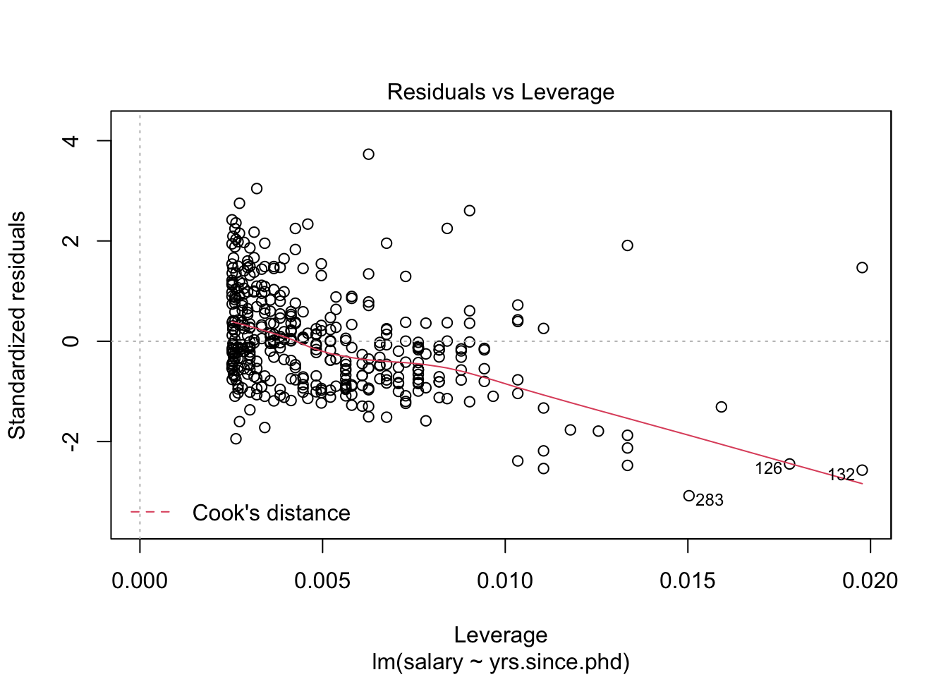
## # .cooksd <dbl>, .std.resid <dbl>We could also use this dataset to plot our residuals, to see if they conform to our conditions. One way to see residual plots is to use the convenience function plot() on our original model object.
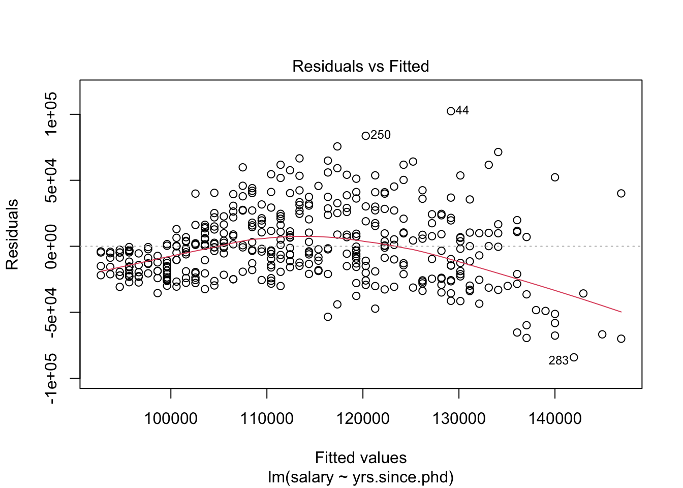
But, a more flexible approach is to create our own residual plots. The augmented data allows us to do this!
ggplot(m1_augmented, aes(x=.fitted, y=.resid)) +
  geom_point() +
  geom_smooth(method = "loess", se=FALSE, formula = "y~x")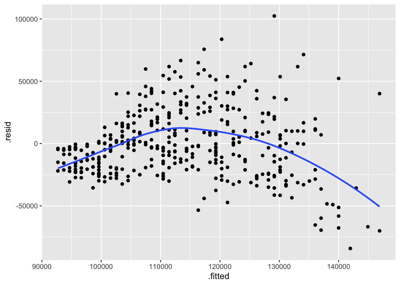
Residual v. fitted plot. Use it to check linearity and equality of variance.
ggplot(Salaries, aes(x=yrs.since.phd, y = salary)) +
  geom_point() +
  geom_smooth(method = "lm", se = FALSE)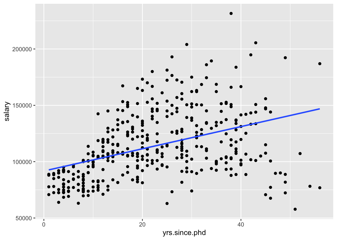
One benefit to making our own residual plots is we can do things like color by a different variable, or facet the plot, to see if there is unexplained variability.
Try coloring the residual v. fitted plot by each of the categorical variables. Which categorical variable do you think explains the most additional variability? How can you tell?
ggplot(m1_augmented, aes(x=.fitted, y=.resid)) +
  geom_point(aes(color = sex)) +
  geom_smooth(method = "loess", se=FALSE, formula = "y~x")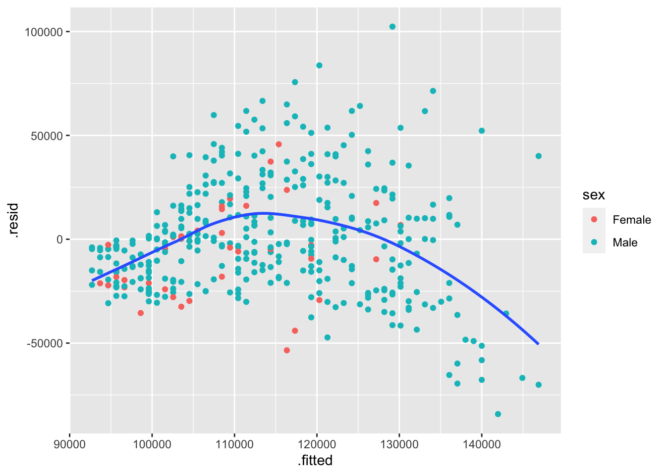
m2 <- lm(log(salary) ~ yrs.since.phd + discipline,
         data = Salaries)
m2_augmented <- augment(m2, data=Salaries)

ggplot(m2_augmented, aes(x=.fitted, y=.resid)) +
  geom_point(aes(color = discipline)) +
  geom_smooth(method = "loess", se=FALSE, formula = "y~x")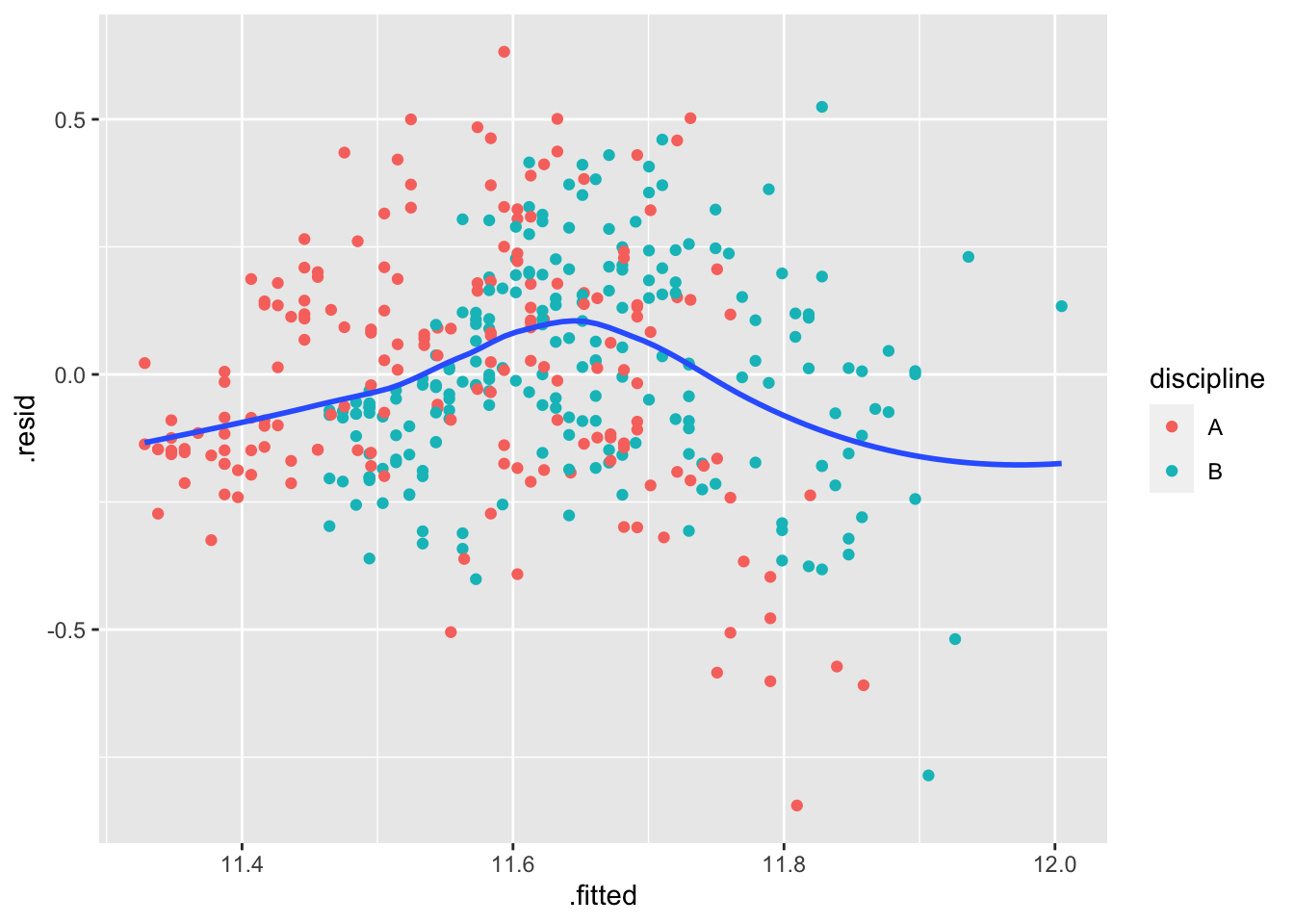
9.4 More dplyr verbs
So far we have learned about filter, select and arrange. Now we want to go into the verbs that modify the data in some way. First, summarize
9.4.1 summarize()
[Note: both the British and American spellings are accepted! I use summarize() most of the time, but summarise() also works.]
This can be thought of as a many-to-one operation. We are moving from many rows of data, and condensing down to just one.
## # A tibble: 1 x 2
##       total   max
##       <int> <int>
## 1 348120517 99686- Use
summarize()to compute three statistics about the data:
- The first (minimum) year in the dataset
- The last (maximum) year in the dataset
- The total number of children represented in the data
There are a few useful helper functions for summarize(),
n(), which counts the number of rows in a dataset or groupn_distinct(), which counts number of distinct values in a variable
Right now, n() doesn’t seem that useful
## # A tibble: 1 x 1
##         n
##     <int>
## 1 1924665
n_distinct() might seem better,
## # A tibble: 1 x 1
##   nname
##   <int>
## 1 97310
But, these become even more useful when combined with…
9.4.2 group_by()
The group_by() function just groups cases by a common value of a particular variable.
## # A tibble: 1,924,665 x 5
## # Groups:   sex [2]
##     year sex   name          n   prop
##    <dbl> <chr> <chr>     <int>  <dbl>
##  1  1880 F     Mary       7065 0.0724
##  2  1880 F     Anna       2604 0.0267
##  3  1880 F     Emma       2003 0.0205
##  4  1880 F     Elizabeth  1939 0.0199
##  5  1880 F     Minnie     1746 0.0179
##  6  1880 F     Margaret   1578 0.0162
##  7  1880 F     Ida        1472 0.0151
##  8  1880 F     Alice      1414 0.0145
##  9  1880 F     Bertha     1320 0.0135
## 10  1880 F     Sarah      1288 0.0132
## # … with 1,924,655 more rows
When combined with other dplyr verbs, it can be very useful!
## # A tibble: 2 x 2
##   sex       total
## * <chr>     <int>
## 1 F     172371079
## 2 M     175749438
9.4.3 mutate()
Our final single-table verb is mutate(). I think of mutate() as a many-to-many transformation. It adds additional columns (variables) to the data.
## # A tibble: 1,924,665 x 6
##     year sex   name          n   prop percent
##    <dbl> <chr> <chr>     <int>  <dbl>   <dbl>
##  1  1880 F     Mary       7065 0.0724    7.24
##  2  1880 F     Anna       2604 0.0267    2.67
##  3  1880 F     Emma       2003 0.0205    2.05
##  4  1880 F     Elizabeth  1939 0.0199    1.99
##  5  1880 F     Minnie     1746 0.0179    1.79
##  6  1880 F     Margaret   1578 0.0162    1.62
##  7  1880 F     Ida        1472 0.0151    1.51
##  8  1880 F     Alice      1414 0.0145    1.45
##  9  1880 F     Bertha     1320 0.0135    1.35
## 10  1880 F     Sarah      1288 0.0132    1.32
## # … with 1,924,655 more rows9.5 More model analysis
Since we have the residuals in m1_augmented, we can use that to compute the sum of squared residuals.
## # A tibble: 1 x 1
##             SSE
##           <dbl>
## 1 299448839521.
Notice that I’m naming my summary statistic, so I could use it later as a variable name.
We can think of partitioning the variability in our response variable as follows,
\[ SST = SSM + SSE \]
where
\[\begin{eqnarray*} SST &=& \sum_{i=1}^n (y_i-\bar{y})^2 \\ SSM &=& \sum_{i=1}^n (\bar{y} - \hat{y})^2 \\ SSE &=& \sum_{i=1}^n (y_i -\hat{y})^2 \end{eqnarray*}\]
Let’s find the other two sums of squares
m1_augmented %>%
  mutate(meansalary = mean(salary)) %>%
  select(salary, .fitted, .resid, meansalary) %>%
  summarize(SSE = sum(.resid^2),
            SSM = sum((meansalary - .fitted)^2),
            SST = sum((salary - meansalary)^2))
## # A tibble: 1 x 3
## SSE SSM SST
## <dbl> <dbl> <dbl>
## 1 299448839521. 63851803040. 363300642561.We don’t have a nice way to interpret those sums of squares, but we can use them to calculate the \(R^2\) value,
\[ R^2 = 1 - \frac{SSE}{SST} = \frac{SSM}{SST} \]
m1_augmented %>%
  mutate(meansalary = mean(salary)) %>%
  summarize(SSE = sum(.resid^2),
            SSM = sum((meansalary - .fitted)^2),
            SST = sum((salary - meansalary)^2)) %>%
  summarize(R2 = 1 - SSE/SST)
## # A tibble: 1 x 1
## R2
## <dbl>
## 1 0.176We can use the \(R^2\) value to assess the model. The larger the \(R^2\) value, the more variability we can explain using the model.
Unfortunately, \(R^2\) always increases as you add predictors, so it is not a good statistic for comparing between models. Instead, we should use adjusted \(R^2\)
\[ R^2_{adj} = 1- \frac{SSE/(n-1)}{SST/(n-k-1)} \]
The adjusted \(R^2\) doesn’t have a nice interpretation, but it can be used to compare between models.
The \(R^2\) and \(R^2_{adj}\) values are given by the model summary table.
##
## Call:
## lm(formula = salary ~ yrs.since.phd, data = Salaries)
##
## Residuals:
##    Min     1Q Median     3Q    Max
## -84171 -19432  -2858  16086 102383
##
## Coefficients:
##               Estimate Std. Error t value Pr(>|t|)
## (Intercept)    91718.7     2765.8  33.162   <2e-16 ***
## yrs.since.phd    985.3      107.4   9.177   <2e-16 ***
## ---
## Signif. codes:  0 '***' 0.001 '**' 0.01 '*' 0.05 '.' 0.1 ' ' 1
##
## Residual standard error: 27530 on 395 degrees of freedom
## Multiple R-squared:  0.1758, Adjusted R-squared:  0.1737
## F-statistic: 84.23 on 1 and 395 DF,  p-value: < 2.2e-16
We can also use the tidy function from broom to tidy up the model coefficients,
## # A tibble: 2 x 5
##   term          estimate std.error statistic   p.value
##   <chr>            <dbl>     <dbl>     <dbl>     <dbl>
## 1 (Intercept)     91719.     2766.     33.2  3.33e-116
## 2 yrs.since.phd     985.      107.      9.18 2.50e- 18
and glance to look at model summaries,
## # A tibble: 1 x 12
##   r.squared adj.r.squared  sigma statistic  p.value    df logLik   AIC   BIC
##       <dbl>         <dbl>  <dbl>     <dbl>    <dbl> <dbl>  <dbl> <dbl> <dbl>
## 1     0.176         0.174 27534.      84.2 2.50e-18     1 -4621. 9248. 9260.
## # … with 3 more variables: deviance <dbl>, df.residual <int>, nobs <int>
Try re-making a few more of our models from yesterday, and glanceing to see which one has the highest adjusted \(R^2\).
library(palmerpenguins)
data("penguins")
library(broom)
favmod <- lm(flipper_length_mm ~ species + bill_depth_mm + body_mass_g + sex, data = penguins)
favmod_augment <- augment(favmod) # works## Error: Assigned data `predict(x, na.action = na.pass, ...) %>% unname()` must be compatible with existing data.
## x Existing data has 344 rows.
## x Assigned data has 333 rows.
## ℹ Only vectors of size 1 are recycled.I didn’t know how to fix this, so I had to look at documentation!
It turns out it has to do with the na.action in lm.
favmod <- lm(flipper_length_mm ~ species + bill_depth_mm + body_mass_g + sex, data = penguins, na.action = "na.exclude")
favmod_augment <- augment(favmod, data = penguins) # works!
Beyond \(R^2\), another useful statistic for assessing a model is the mean squared error, or the root mean squared error
\[
MSE = \frac{1}{n}\sum_{i=1}^n (y_i-\hat{y}_i)^2 \\
RMSE = \sqrt{MSE}
\]
Try using dplyr verbs to compure the RMSE.
9.6 Bonus: comment on theory!
Although we are trying to “minimize” the sum of squared residuals, we don’t have to use a simulation method. Regression is actually done using matrix operations.
Suppose we have a sample of \(n\) subjects. For subject \(i\in{1,...,n}\) let \(Y_i\) denote the observed response value and \((x_{i1},x_{i2},\dots,x_{ik})\) denote the observed values of the \(k\) predictors. Then we can collect our observed response values into a vector \(y\), our predictor values into a matrix \(X\), and our regression coefficients into a vector \(\beta\). Note that a column of 1s is included for an intercept term in \(X\):
\[\begin{eqnarray*}y= \begin{pmatrix} y_1 \\ y_2 \\ \vdots \\ y_n \end{pmatrix}, X = \begin{pmatrix} 1 & x_{11} x_{12} \dots x_{1k} \\ 1 & x_{21} & x_{22} & \dots x_{2k} \\ \vdots & \vdots & \vdots & \dots & \vdots \\ 1 & x_{n1} & x_{n2} & \dots & x_{nk} \end{pmatrix}, \text{ and } \beta = \begin{pmatrix} beta_1 \\ \beta_2 \\ \vdots \\ \beta_k \end{pmatrix} \end{eqnarray*}\]
Then we can express the model \(y_i=\beta_0+\beta_1 x_{i1}+\dots +\beta_{k}x_{ik}\) for \(i\in{1,\dots,n}\) using linear algebra:
\[ y=X\beta \] Further, let \(\hat{\beta}\) denote the vector of sample estimated \(\hat{beta}\), and \(\hat{y}\) denote the vector of predictions/model values:
\[ \hat{y}=X\hat{\beta} \] Thus the residual vector is \[ y−\hat{y}=X\beta−X\hat{\beta} \] and the sum of squared residuals is \[ (y−\hat{y})^T(y−\hat{y}) \] Challenge: Prove that the following formula for sample coefficients \(\beta\) are the least squares estimates of \(\beta\), ie. they minimize the sum of squared residuals: \[ \hat{\beta}=(X^TX)^{-1}X^Ty \]