Chapter 6 Logistic Regression
6.1 Logistic Regression
6.1.1 Modeling Binary Response
So far, we have modeled only quantitative response variables.
The normal error regression model makes the assumption that the response variable is normally distributed, given the value(s) of the explanatory variables.
Now, we’ll look at how to model a categorical response variable. We’ll consider only situations where the response is binary (i.e. has 2 categories)
6.1.2 Credit Card Dataset
We’ll consider a dataset pertaining to 10,000 credit cards. The goal is to predict whether or not the user will default on the payment, using information on the credit card balance, user’s annual income, and whether or not the user is a student. Data come from Introduction to Statistical Learning by James, Witten, Hastie, Tibshirani.
library(ISLR)
data(Default)
summary(Default)
## default student balance income
## No :9667 No :7056 Min. : 0.0 Min. : 772
## Yes: 333 Yes:2944 1st Qu.: 481.7 1st Qu.:21340
## Median : 823.6 Median :34553
## Mean : 835.4 Mean :33517
## 3rd Qu.:1166.3 3rd Qu.:43808
## Max. :2654.3 Max. :735546.1.3 Default and Balance
ggplot(data=Default, aes(y=default, x=balance)) + geom_point(alpha=0.2) 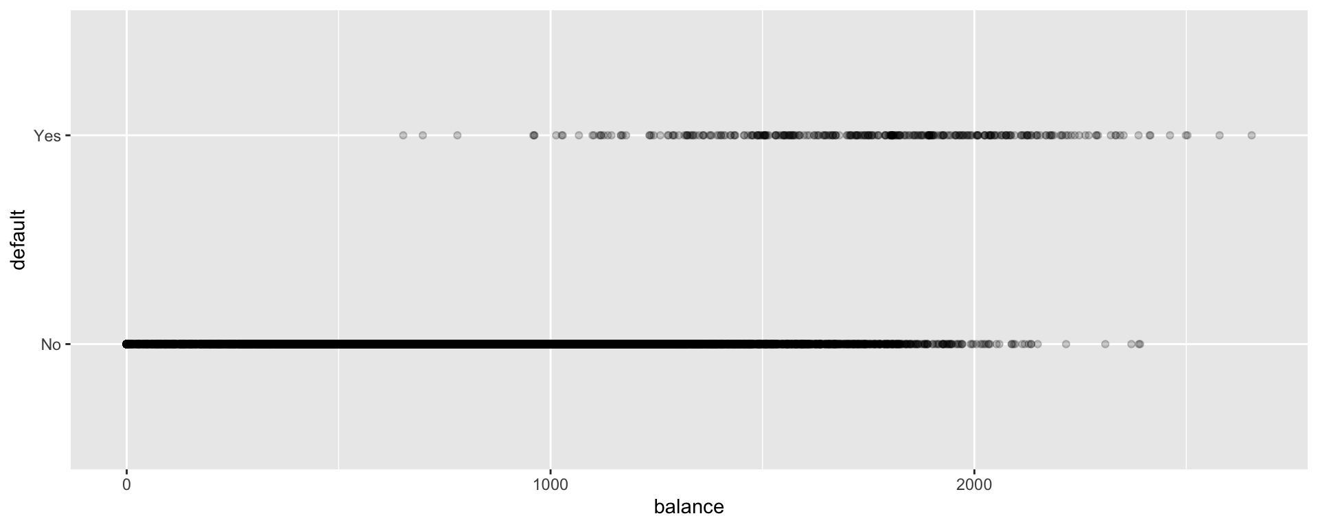
6.1.4 Linear Regression Model for Education Level
#convert default from yes/no to 0/1
Default$default <- as.numeric(Default$default=="Yes") ggplot(data=Default, aes(y=default, x= balance)) + geom_point(alpha=0.2) + stat_smooth(method="lm", se=FALSE)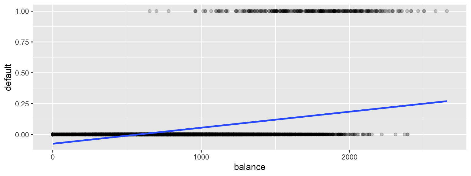
There are a lot of problems with this model!
6.1.5 Transforming into interval (0,1)
Starting with our linear model \(E(Y_i) = \beta_0+\beta_1x_{i1}\), we need to transform \(\beta_0+\beta_1x_{i1}\) into (0,1).
Let \(\pi_i = \frac{e^{\beta_0+\beta_1x_{i1} }}{1+e^{\beta_0+\beta_1x_{i1}}}\).
Then \(0 \leq \pi_i \leq 1\), and \(\pi_i\) represents an estimate of \(P(Y_i=1)\).
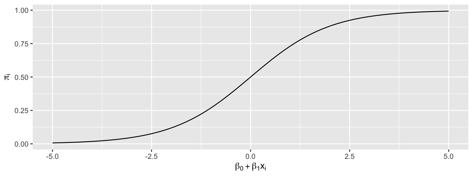
This function maps the values of \(\beta_0+\beta_1x_{i1}\) into the interval (0,1).
The logistic regression model assumes that:
- \(Y_i \in \{0,1\}\)
- \(E(Y_i) = P(Y_i=1) = \pi_i=\frac{e^{\beta_0+\beta_1x_{i1} + \ldots \beta_px_{ip}}}{1+e^{\beta_0+\beta_1x_{i1} + \ldots \beta_px_{ip}}}\)
- \(Y_i \in \{0,1\}\)
i.e. \(\beta_0+\beta_1x_{i1} + \ldots \beta_px_{ip}= \text{log}\left(\frac{\pi_i}{1-\pi_i}\right).\) (This is called the logit function and can be written \(\text{logit}(\pi_i)\).
- Instead of assuming that the expected response is a linear function of the explanatory variables, we are assuming that it is a function of a linear function of the explanatory variables.
6.1.6 Logistic Regression Model for Balance
ggplot(data=Default, aes(y=default, x= balance)) + geom_point(alpha=0.2) +
stat_smooth(method="glm", se=FALSE, method.args = list(family=binomial)) 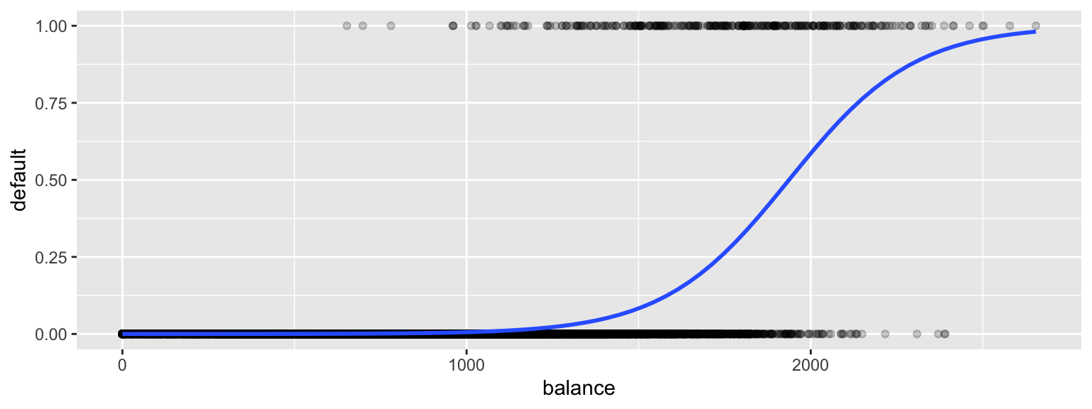
6.1.7 Fitting the Logistic Regression Model in R
CCDefault_M <- glm(data=Default, default ~ balance, family = binomial(link = "logit"))
summary(CCDefault_M)
##
## Call:
## glm(formula = default ~ balance, family = binomial(link = "logit"),
## data = Default)
##
## Deviance Residuals:
## Min 1Q Median 3Q Max
## -2.2697 -0.1465 -0.0589 -0.0221 3.7589
##
## Coefficients:
## Estimate Std. Error z value Pr(>|z|)
## (Intercept) -10.6513306 0.3611574 -29.49 <0.0000000000000002 ***
## balance 0.0054989 0.0002204 24.95 <0.0000000000000002 ***
## ---
## Signif. codes: 0 '***' 0.001 '**' 0.01 '*' 0.05 '.' 0.1 ' ' 1
##
## (Dispersion parameter for binomial family taken to be 1)
##
## Null deviance: 2920.6 on 9999 degrees of freedom
## Residual deviance: 1596.5 on 9998 degrees of freedom
## AIC: 1600.5
##
## Number of Fisher Scoring iterations: 86.1.8 The Logistic Regression Equation
The regression equation is:
\[ P(\text{Default}) = \hat{\pi}_i = \frac{e^{-10.65+0.0055\times\text{balance}}}{1+e^{-10.65+0.0055\times\text{balance}}} \]
For a $1,000 balance, the estimated default probability is \(\frac{e^{-10.65+0.0055(1000) }}{1+e^{-10.65+0.0055(1000)}} \approx 0.006\)
For a $1,500 balance, the estimated default probability is \(\frac{e^{-10.65+0.0055(1500) }}{1+e^{-10.65+0.0055(1500)}} \approx 0.08\)
For a $2,000 balance, the estimated default probability is \(\frac{e^{-10.65+0.0055(2000) }}{1+e^{-10.65+0.0055(2000)}} \approx 0.59\)
6.1.9 Predict in R
predict(CCDefault_M, newdata=data.frame((balance=1000)), type="response")## 1
## 0.005752145predict(CCDefault_M, newdata=data.frame((balance=1500)), type="response")## 1
## 0.08294762predict(CCDefault_M, newdata=data.frame((balance=2000)), type="response")## 1
## 0.58576946.1.10 Where do the b’s come from?
Recall that for a quantitative response variable, the values of \(b_1, b_2, \ldots, b_p\) are chosen in a way that minimizes \(\displaystyle\sum_{i=1}^n \left(y_i-(\beta_0+\beta_1x_{i1}+\ldots+\beta_px_{ip})^2\right)\).
Least squares does not work well in this generalized setting. Instead, the b’s are calculated using a more advanced technique, known as maximum likelihood estimation.
6.2 Interpretations in a Logistic Regression Model
6.2.1 Recall Logistic Regression Curve for Credit Card Data
ggplot(data=Default, aes(y=default, x= balance)) + geom_point(alpha=0.2) +
stat_smooth(method="glm", se=FALSE, method.args = list(family=binomial)) 
6.2.2 Recall Credit Card Model Output
M <- glm(data=Default, default ~ balance, family = binomial(link = "logit"))
summary(M)
##
## Call:
## glm(formula = default ~ balance, family = binomial(link = "logit"),
## data = Default)
##
## Deviance Residuals:
## Min 1Q Median 3Q Max
## -2.2697 -0.1465 -0.0589 -0.0221 3.7589
##
## Coefficients:
## Estimate Std. Error z value Pr(>|z|)
## (Intercept) -10.6513306 0.3611574 -29.49 <0.0000000000000002 ***
## balance 0.0054989 0.0002204 24.95 <0.0000000000000002 ***
## ---
## Signif. codes: 0 '***' 0.001 '**' 0.01 '*' 0.05 '.' 0.1 ' ' 1
##
## (Dispersion parameter for binomial family taken to be 1)
##
## Null deviance: 2920.6 on 9999 degrees of freedom
## Residual deviance: 1596.5 on 9998 degrees of freedom
## AIC: 1600.5
##
## Number of Fisher Scoring iterations: 86.2.3 Balance Logistic Model Equation
The regression equation is:
\[ P(\text{Default}) = \hat{\pi}_i = \frac{e^{-10.65+0.0055\times\text{balance}}}{1+e^{-10.65+0.0055\times\text{balance}}} \]
For a $1,000 balance, the estimated default probability is \(\hat{\pi}_i=\frac{e^{10.65+0.0055(1000) }}{1+e^{10.65+0.0055(1000)}} \approx 0.005752145\)
For a $1,500 balance, the estimated default probability is \(\hat{\pi}_i=\frac{e^{10.65+0.0055(1500) }}{1+e^{10.65+0.0055(1500)}} \approx 0.08294762\)
For a $2,000 balance, the estimated default probability is \(\hat{\pi}_i=\frac{e^{10.65+0.0055(2000) }}{1+e^{10.65+0.0055(2000)}} \approx 0.5857694\)
6.2.4 Odds
For an event with probability \(p\), the odds of the event occurring are \(\frac{p}{1-p}\).
The odds of default are given by \(\frac{\pi_i}{1-\pi_i}\).
Examples:
The estimated odds of default for a $1,000 balance are \(\frac{0.005752145}{1-0.005752145} \approx 1:173.\)
The estimated odds of default for a $1,500 balance are \(\frac{0.08294762 }{1-0.08294762 } \approx 1:11.\)
The estimated odds of default for a $2,000 balance are \(\frac{0.5857694}{1-0.5857694} \approx 1.414:1.\)
6.2.5 Odds Ratio
The quantity \(\frac{\frac{\pi_i}{1-\pi_i}}{\frac{\pi_j}{1-\pi_j}}\) represents the odds ratio of a default for user \(i\), compared to user \(j\). This quantity is called the odds ratio.
Example:
The default odds ratio for a $1,000 payment, compared to a $2,000 payment is
The odds ratio is \(\frac{\frac{1}{173}}{\frac{1.414}{1}}\approx 1:244.\)
The odds of a default are about 244 times larger for a $2,000 payment than a $1,000 payment.
6.2.6 Interpretation of \(\beta_1\)
Consider the odds ratio for a case \(j\) with explanatory variable \(x + 1\), compared to case \(i\) with explanatory variable \(x\).
That is \(\text{log}\left(\frac{\pi_i}{1-\pi_i}\right) = \beta_0+\beta_1x\), and \(\text{log}\left(\frac{\pi_j}{1-\pi_j}\right) = \beta_0+\beta_1(x+1)\).
\(\text{log}\left(\frac{\frac{\pi_j}{1-\pi_j}}{\frac{\pi_i}{1-\pi_i}}\right)=\text{log}\left(\frac{\pi_j}{1-\pi_j}\right)-\text{log}\left(\frac{\pi_i}{1-\pi_j}\right)=\beta_0+\beta_1(x+1)-(\beta_0+\beta_1(x))=\beta_1.\)
Thus a 1-unit increase in \(x\) is associated with a multiplicative change in the log odds by a factor of \(\beta_1\).
A 1-unit increase in \(x\) is associated with a multiplicative change in the odds by a factor of \(e^{\beta_1}\).
6.2.7 Intrepretation in Credit Card Example
\(b_1=0.0055\)
The odds of default are estimated to multiply by \(e^{0.0055}\approx1.0055\) for each 1-dollar increase in balance on the credit card.
That is, the odds of default are estimated to increase by 0.55% for each additional dollar on the card balance.
An increase of \(d\) dollars in credit card balance is estimated to be associated with an increase odds of default by a factor of \(e^{0.0055d}\).
The odds of default for a balance of $2,000 are estimated to be \(e^{0.0055\times 1000}\approx 244\) times as great as the odds of default for a $1,000 balance.
6.2.8 Hypothesis Tests in Logistic Regression
The p-value on the “balance” line of the regression output is associated with the null hypothesis \(\beta_1=0\), that is that there is no relationship between balance and the odds of defaulting on the payment.
The fact that the p-value is so small tells us that there is strong evidence of a relationship between balance and odds of default.
6.2.9 Confidence Intervals for \(\beta_1\)
confint(M, level = 0.95)## 2.5 % 97.5 %
## (Intercept) -11.383288936 -9.966565064
## balance 0.005078926 0.005943365We are 95% confident that a 1 dollar increase in credit card balance is associate with an increased odds of default by a factor between \(e^{0.00508}\approx 1.0051\) and \(e^{0.00594}\approx 1.0060\).
This is a profile-likelihood interval, which you can read more about here.
6.3 Multiple Logistic Regression
6.3.1 Logistic Regression Models with Multiple Explanatory Variables
We can also perform logistic regression in situations where there are multiple explanatory variables.
6.3.2 Logistic Model with Multiple Predictors
CCDefault_M2 <- glm(data=Default, default ~ balance + student, family = binomial(link = "logit"))
summary(CCDefault_M2)
##
## Call:
## glm(formula = default ~ balance + student, family = binomial(link = "logit"),
## data = Default)
##
## Deviance Residuals:
## Min 1Q Median 3Q Max
## -2.4578 -0.1422 -0.0559 -0.0203 3.7435
##
## Coefficients:
## Estimate Std. Error z value Pr(>|z|)
## (Intercept) -10.7494959 0.3691914 -29.116 < 0.0000000000000002 ***
## balance 0.0057381 0.0002318 24.750 < 0.0000000000000002 ***
## studentYes -0.7148776 0.1475190 -4.846 0.00000126 ***
## ---
## Signif. codes: 0 '***' 0.001 '**' 0.01 '*' 0.05 '.' 0.1 ' ' 1
##
## (Dispersion parameter for binomial family taken to be 1)
##
## Null deviance: 2920.6 on 9999 degrees of freedom
## Residual deviance: 1571.7 on 9997 degrees of freedom
## AIC: 1577.7
##
## Number of Fisher Scoring iterations: 86.3.3 Multiple Logistic Model Illustration
ggplot(data=Default, aes(y=default, x= balance, color=student)) + geom_point(alpha=0.2) + stat_smooth(method="glm", se=FALSE, method.args = list(family=binomial)) 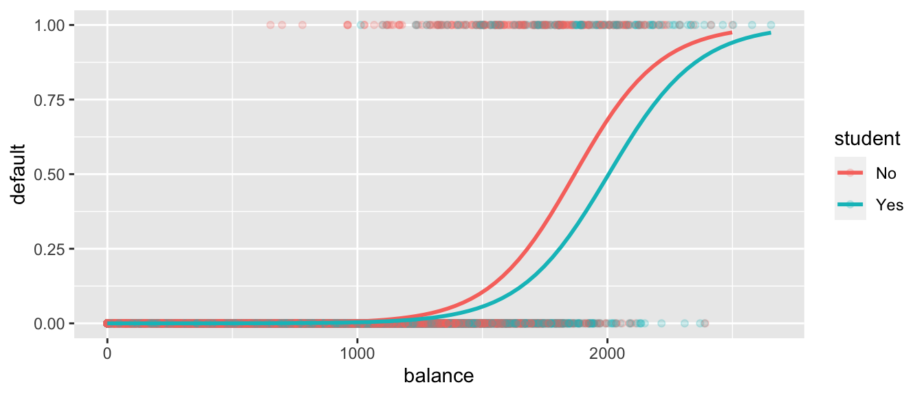
6.3.4 Multiple Logistic Regression Interpretation
The regression equation is:
\[ P(\text{Default}) = \hat{\pi}_i = \frac{e^{-10.75+0.00575\times\text{balance}-0.7149\times\text{I}_{\text{student}}}}{1+e^{-10.75+0.00575\times\text{balance}-0.7149\times\text{I}_{\text{student}}}} \]
The odds of default are estimated to multiply by \(e^{0.005738}\approx 1.00575\) for each 1 dollar increase in balance whether the user is a student or nonstudent. Thus, the estimated odds of default increase by about 0.05%.
We might be more interested in what would happen with a larger increase, say $100. The odds of default are estimated to multiply by \(e^{0.005738\times100}\approx 1.775\) for each $100 increase in balance for students as well as nonstudents. Thus, the estimated odds of default increase by about 77.5%.
The odds of default for students are estimated to be \(e^{-0.7149} \approx 0.49\) as high for students as non-students, assuming balance amount is held constant.
6.3.5 Hypothesis Tests in Multiple Logistic Regression Model
There is strong evidence of a relationship between balance and odds of default, provided we are comparing students to students, or nonstudents to nonstudents.
There is evidence that students are less likely to default than nonstudents, provided the balance on the card is the same.
6.3.6 Multiple Logistic Regression Model with Interaction
CCDefault_M_Int <- glm(data=Default, default ~ balance * student, family = binomial(link = "logit"))
summary(CCDefault_M_Int)
##
## Call:
## glm(formula = default ~ balance * student, family = binomial(link = "logit"),
## data = Default)
##
## Deviance Residuals:
## Min 1Q Median 3Q Max
## -2.4839 -0.1415 -0.0553 -0.0202 3.7628
##
## Coefficients:
## Estimate Std. Error z value Pr(>|z|)
## (Intercept) -10.8746818 0.4639679 -23.438 <0.0000000000000002 ***
## balance 0.0058188 0.0002937 19.812 <0.0000000000000002 ***
## studentYes -0.3512310 0.8037333 -0.437 0.662
## balance:studentYes -0.0002196 0.0004781 -0.459 0.646
## ---
## Signif. codes: 0 '***' 0.001 '**' 0.01 '*' 0.05 '.' 0.1 ' ' 1
##
## (Dispersion parameter for binomial family taken to be 1)
##
## Null deviance: 2920.6 on 9999 degrees of freedom
## Residual deviance: 1571.5 on 9996 degrees of freedom
## AIC: 1579.5
##
## Number of Fisher Scoring iterations: 86.3.7 Interpretations for Logistic Model with Interaction
- The regression equation is:
\[ P(\text{Default}) = \hat{\pi}_i = \frac{e^{-10.87+0.0058\times\text{balance}-0.35\times\text{I}_{\text{student}}-0.0002\times\text{balance}\times{\text{I}_{\text{student}}}}}{1+e^{-10.87+0.0058\times\text{balance}-0.35\times\text{I}_{\text{student}}-0.0002\times\text{balance}\times{\text{I}_{\text{student}}}}} \]
- Since estimate of the interaction effect is so small and the p-value on this estimate is large, it is plausible that there is no interaction at all. Thus, the simpler non-interaction model is preferable.
6.3.8 Logistic Regression Key Points
\(Y\) is a binary response variable.
\(\pi_i\) is a function of explanatory variables \(x_{i1}, \ldots x_{ip}\).
\(E(Y_i) = \pi_i = \frac{e^{\beta_0+\beta_1x_i + \ldots\beta_px_{ip}}}{1+e^{\beta_0+\beta_1x_i + \ldots\beta_px_{ip}}}\)
\(\beta_0+\beta_1x_i + \ldots\beta_px_{ip} = \text{log}\left(\frac{\pi_i}{1-\pi_i}\right)\)
For quantitative \(x_j\), when all other explanatory variables are held constant, the odds of “success” multiply be a factor of \(e^\beta_j\) for each 1 unit increase in \(x_j\)
For categorical \(x_j\), when all other explanatory variables are held constant, the odds of “success” are \(e^\beta_j\) times higher for category \(j\) than for the “baseline category.”
For models with interaction, we can only interpret \(\beta_j\) when the values of all other explanatory variables are given (since the effect of \(x_j\) depends on the other variables.)