Chapter 8 Building Models for Prediction
8.1 Training and Test Error
8.1.1 Modeling for the Purpose of Prediction
- When our purpose is purely prediction, we don’t need to worry about keeping the model simple enough to interpret.
- Goal is to fit data well enough to make good predictions on new data without modeling random noise (overfitting)
- A model that is too simple suffers from high bias
- A model that is too complex suffers from high variance and is prone to overfitting
- The right balance is different for every dataset
- Measuring error on data used to fit the model (training data) does not accurately predict how well model will be able to predict new data (test data)
8.1.2 Model for Predicting Car Price
Consider the following five models for predicting the price of a new car. The models are fit, using the sample of 110 cars released in 2015, that we’ve seen previously.
M1 <- lm(data=Cars2015, LowPrice~Acc060)
M2 <- lm(data=Cars2015, LowPrice~Acc060 + I(Acc060^2))
M3 <- lm(data=Cars2015, LowPrice~Acc060 + I(Acc060^2) + Size)
M4 <- lm(data=Cars2015, LowPrice~Acc060 + I(Acc060^2) + Size + PageNum)
M5 <- lm(data=Cars2015, LowPrice~Acc060 * I(Acc060^2) * Size)
M6 <- lm(data=Cars2015, LowPrice~Acc060 * I(Acc060^2) * Size * PageNum)
Which would perform best if we were making predictions on a different set of cars, released in 2015?
8.1.3 Prediction Simulation Example
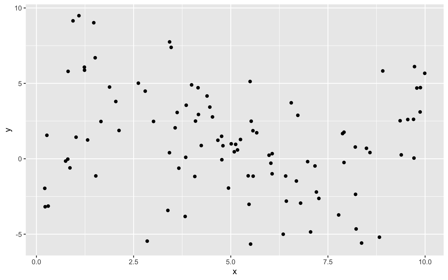
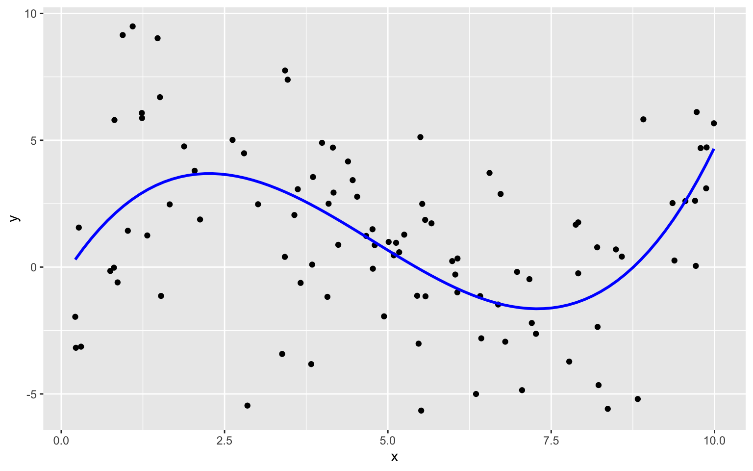
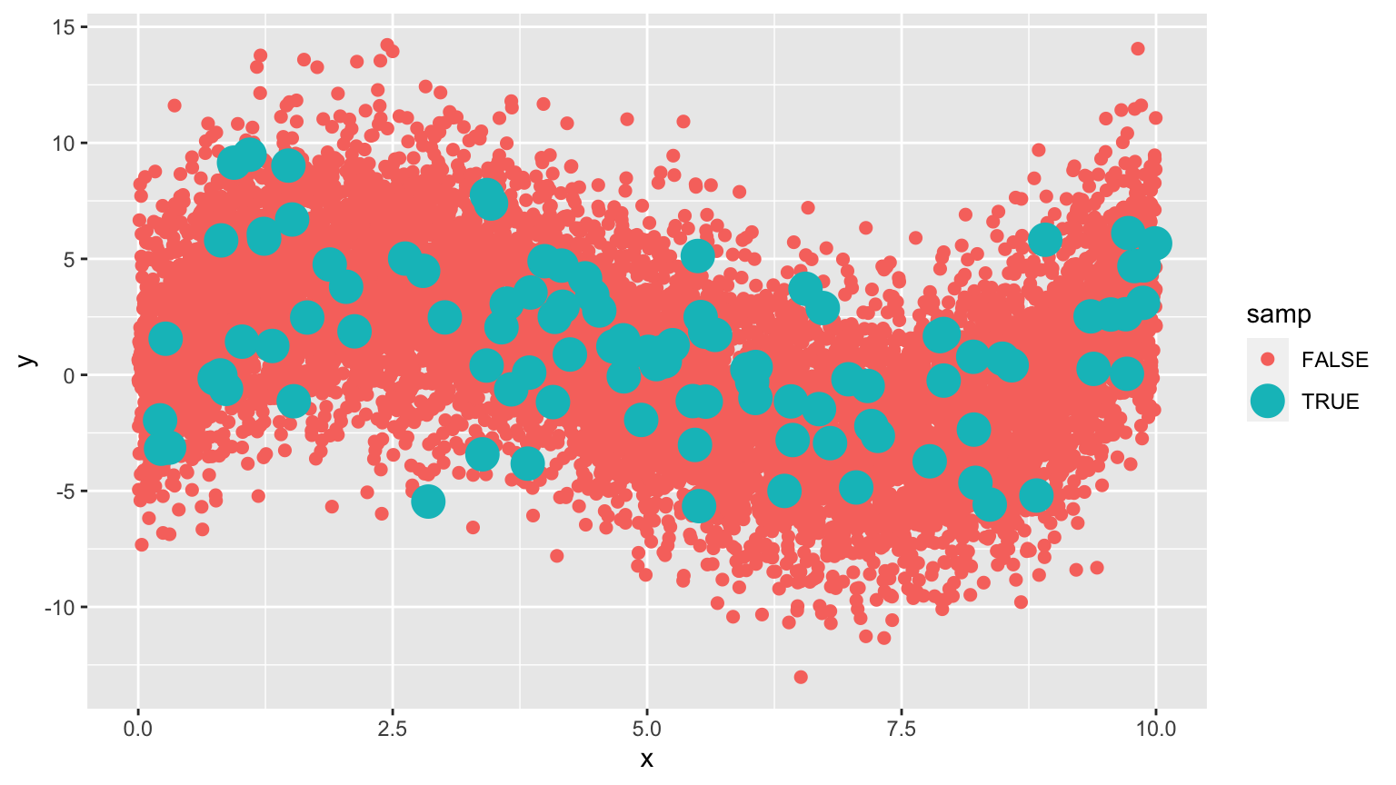
Suppose we have a set of 100 observations of a single explanatory variable \(x\), and response variable \(y\). A scatterplot of the data is shown below.
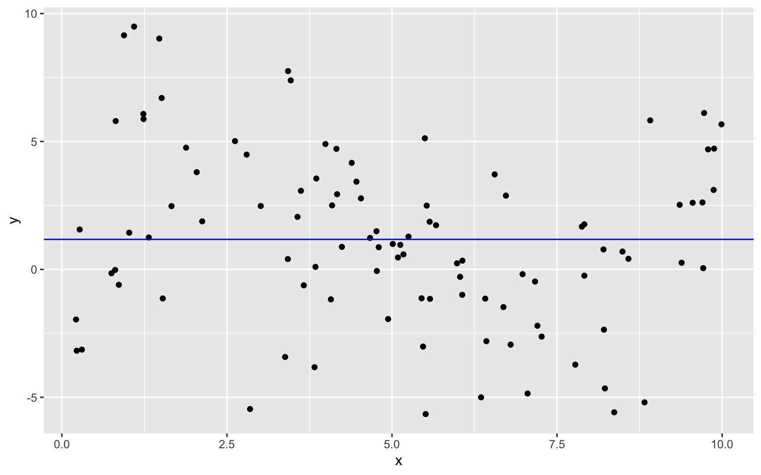
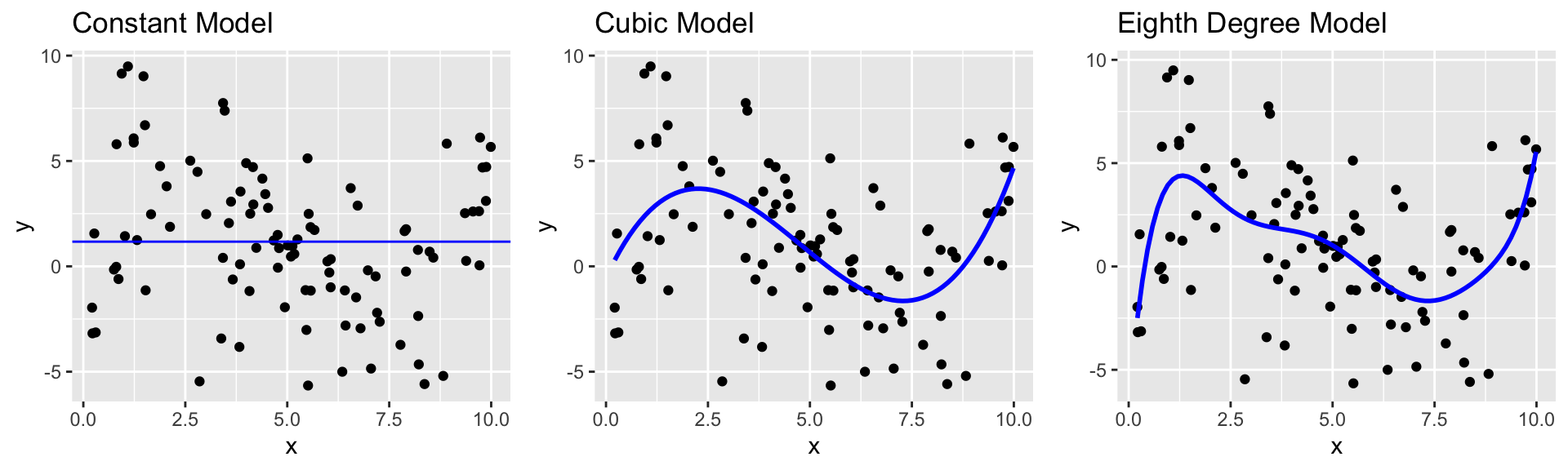
8.1.4 Constant Model to Sample Data
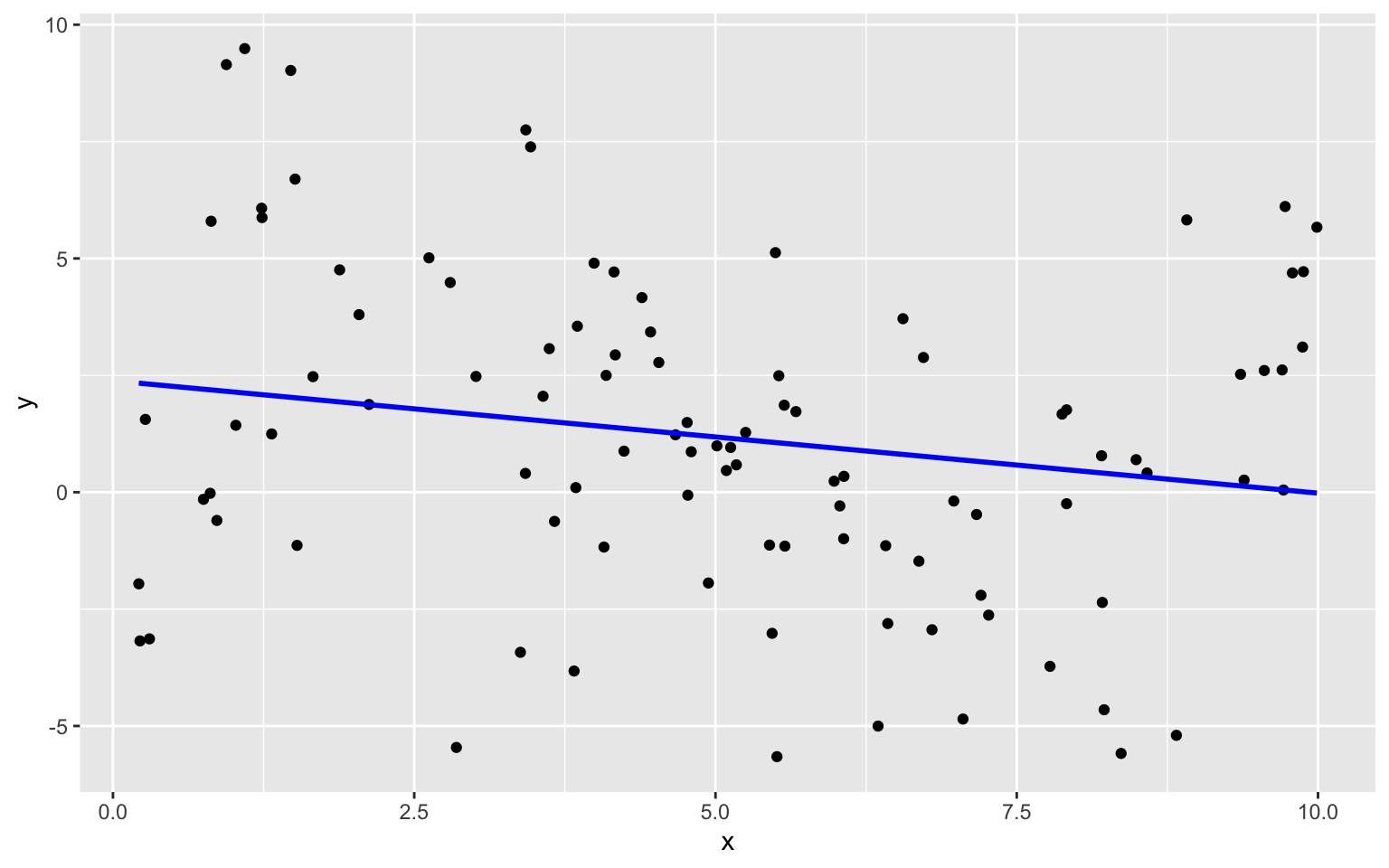
8.1.5 Linear Model to Sample Data
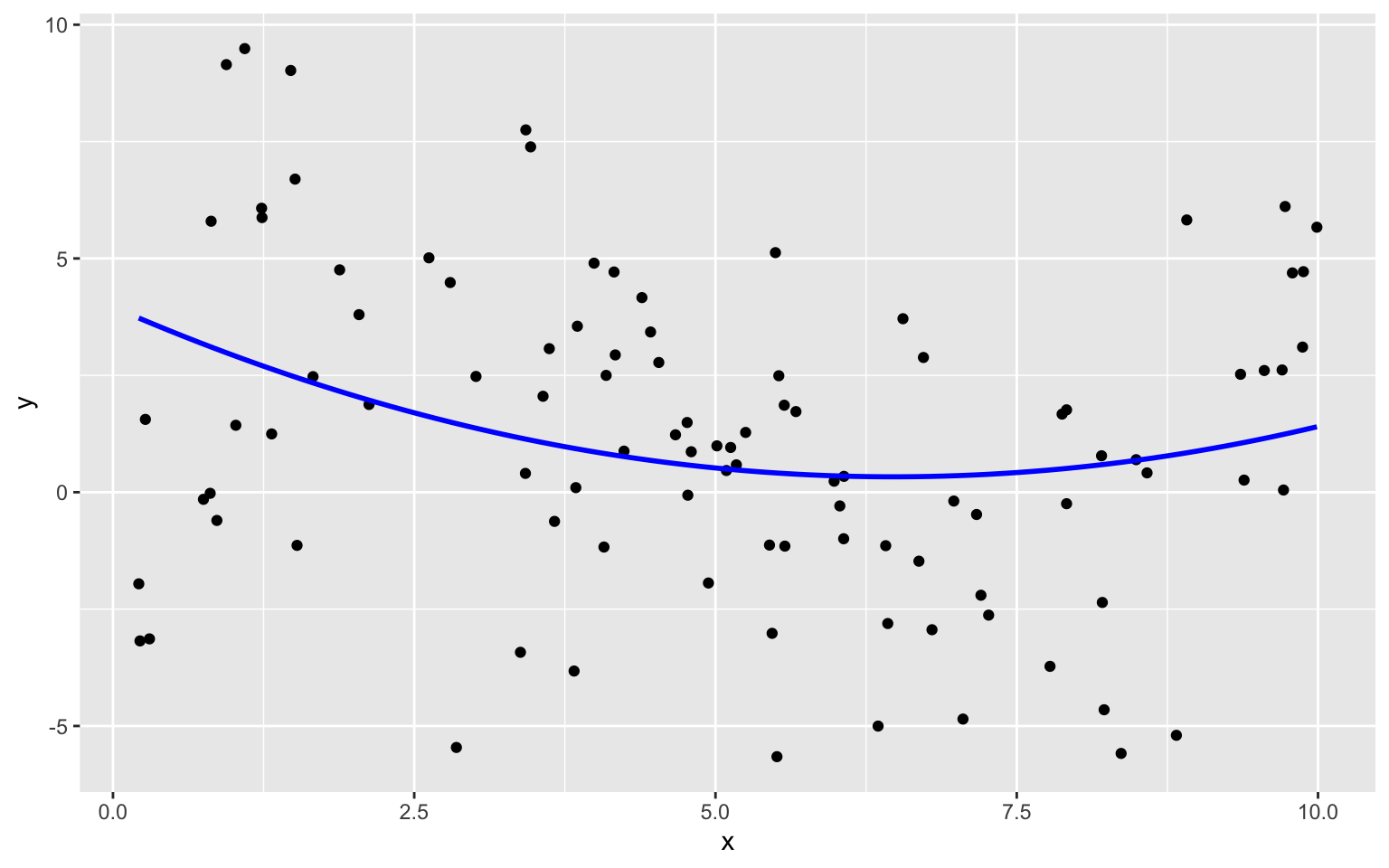
8.1.6 Quadratic Model
8.1.7 Cubic Model
8.1.8 Quartic Model
8.1.9 Degree 8 Model
8.1.10 Model Complexity
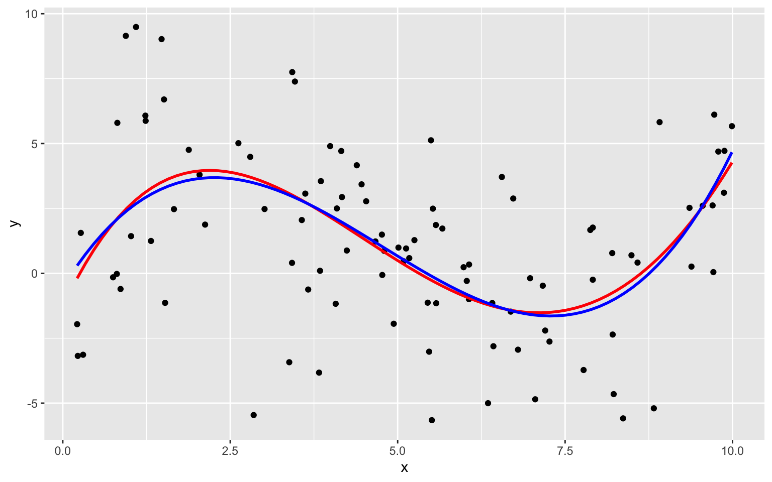
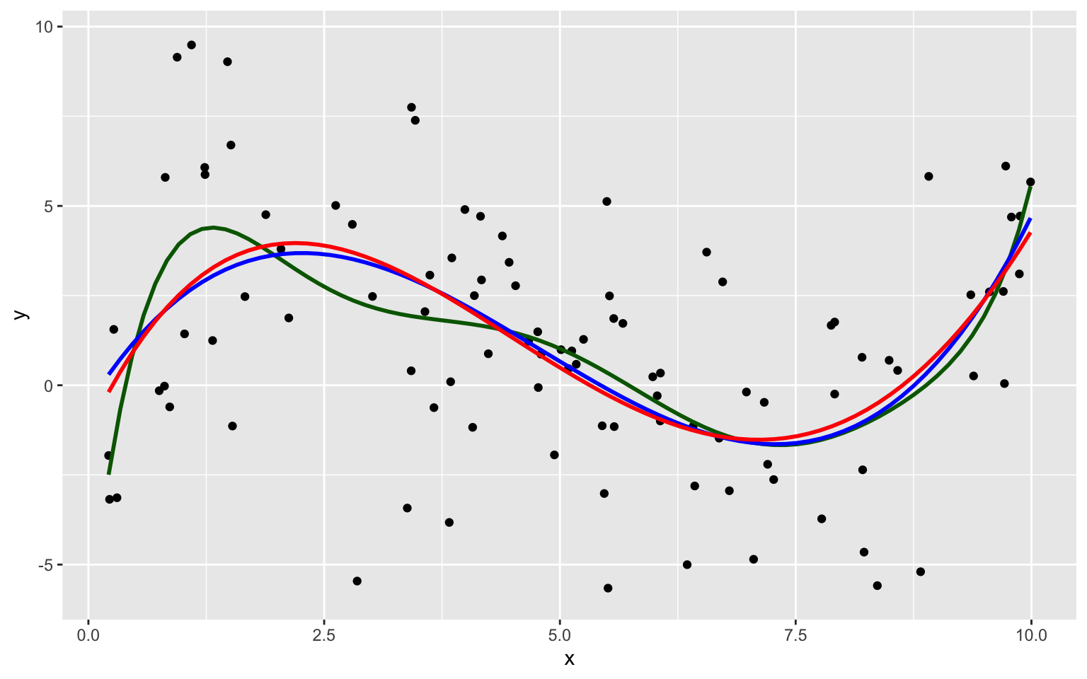
The complexity of the model increases as we add higher-order terms. This makes the model more flexible. The curve is allowed to have more twists and bends.
For higher-order, more complex models, individual points have more influence on the shape of the curve.
8.1.11 New Data for Prediction
Now, suppose we have a new dataset of 100, x-values, and want to predict \(y\). The first 5 rows of the new dataset are shown
| x | Prediction |
|---|---|
| 3.196237 | ? |
| 1.475586 | ? |
| 5.278882 | ? |
| 5.529299 | ? |
| 7.626731 | ? |
8.1.12 Fit Polynomial Models
Sim_M0 <-lm(data=Sampdf, y~1)
Sim_M1 <-lm(data=Sampdf, y~x)
Sim_M2 <- lm(data=Sampdf, y~x+I(x^2))
Sim_M3 <- lm(data=Sampdf, y~x+I(x^2)+I(x^3))
Sim_M4 <- lm(data=Sampdf, y~x+I(x^2)+I(x^3)+I(x^4))
Sim_M5 <- lm(data=Sampdf, y~x+I(x^2)+I(x^3)+I(x^4)+I(x^5))
Sim_M6 <- lm(data=Sampdf, y~x+I(x^2)+I(x^3)+I(x^4)+I(x^5)+I(x^6))
Sim_M7 <- lm(data=Sampdf, y~x+I(x^2)+I(x^3)+I(x^4)+I(x^5)+I(x^6)+I(x^7))
Sim_M8 <- lm(data=Sampdf, y~x+I(x^2)+I(x^3)+I(x^4)+I(x^5)+I(x^6)+I(x^7)+I(x^8))
8.1.13 Predictions for New Data
Newdf$Deg0Pred <- predict(Sim_M0, newdata=Newdf)
Newdf$Deg1Pred <- predict(Sim_M1, newdata=Newdf)
Newdf$Deg2Pred <- predict(Sim_M2, newdata=Newdf)
Newdf$Deg3Pred <- predict(Sim_M3, newdata=Newdf)
Newdf$Deg4Pred <- predict(Sim_M4, newdata=Newdf)
Newdf$Deg5Pred <- predict(Sim_M5, newdata=Newdf)
Newdf$Deg6Pred <- predict(Sim_M6, newdata=Newdf)
Newdf$Deg7Pred <- predict(Sim_M7, newdata=Newdf)
Newdf$Deg8Pred <- predict(Sim_M8, newdata=Newdf)
8.1.14 Predicted Values
kable(Newdf %>% dplyr::select(-c(y, samp)) %>% round(2) %>% head(5))| x | Deg0Pred | Deg1Pred | Deg2Pred | Deg3Pred | Deg4Pred | Deg5Pred | Deg6Pred | Deg7Pred | Deg8Pred | |
|---|---|---|---|---|---|---|---|---|---|---|
| 108 | 5.53 | 1.17 | 1.05 | 0.41 | -0.14 | -0.30 | 0.10 | 0.40 | 0.25 | 0.31 |
| 4371 | 2.05 | 1.17 | 1.89 | 2.02 | 3.66 | 3.95 | 4.26 | 3.82 | 3.37 | 3.49 |
| 4839 | 3.16 | 1.17 | 1.63 | 1.29 | 3.24 | 3.35 | 2.78 | 2.24 | 2.15 | 2.07 |
| 6907 | 2.06 | 1.17 | 1.89 | 2.02 | 3.66 | 3.95 | 4.25 | 3.80 | 3.36 | 3.47 |
| 7334 | 2.92 | 1.17 | 1.68 | 1.42 | 3.43 | 3.60 | 3.14 | 2.51 | 2.31 | 2.25 |
8.1.15 Predicted Values and True y
In fact, since these data were simulated, we know the true value of \(y\).
kable(Newdf %>% dplyr::select(-c(samp)) %>% round(2) %>% head(5))| x | y | Deg0Pred | Deg1Pred | Deg2Pred | Deg3Pred | Deg4Pred | Deg5Pred | Deg6Pred | Deg7Pred | Deg8Pred | |
|---|---|---|---|---|---|---|---|---|---|---|---|
| 108 | 5.53 | 5.49 | 1.17 | 1.05 | 0.41 | -0.14 | -0.30 | 0.10 | 0.40 | 0.25 | 0.31 |
| 4371 | 2.05 | 3.92 | 1.17 | 1.89 | 2.02 | 3.66 | 3.95 | 4.26 | 3.82 | 3.37 | 3.49 |
| 4839 | 3.16 | 1.46 | 1.17 | 1.63 | 1.29 | 3.24 | 3.35 | 2.78 | 2.24 | 2.15 | 2.07 |
| 6907 | 2.06 | 6.79 | 1.17 | 1.89 | 2.02 | 3.66 | 3.95 | 4.25 | 3.80 | 3.36 | 3.47 |
| 7334 | 2.92 | -1.03 | 1.17 | 1.68 | 1.42 | 3.43 | 3.60 | 3.14 | 2.51 | 2.31 | 2.25 |
8.1.16 Evaluating Predictions - RMSE
For quantitative response variables, we can evaluate the predictions by calculating the average of the squared differences between the true and predicted values. Often, we look at the square root of this quantity. This is called the Root Mean Square Prediction Error (RMSPE).
\[ \text{RMSPE} = \sqrt{\displaystyle\sum_{i=1}^{n'}\frac{(y_i-\hat{y}_i)^2}{n'}}, \]
where \(n'\) represents the number of new cases being predicted.
8.1.17 Calculate Prediction Error
RMSPE0 <- sqrt(mean((Newdf$y-Newdf$Deg0Pred)^2))
RMSPE1 <- sqrt(mean((Newdf$y-Newdf$Deg1Pred)^2))
RMSPE2 <- sqrt(mean((Newdf$y-Newdf$Deg2Pred)^2))
RMSPE3 <- sqrt(mean((Newdf$y-Newdf$Deg3Pred)^2))
RMSPE4 <- sqrt(mean((Newdf$y-Newdf$Deg4Pred)^2))
RMSPE5 <- sqrt(mean((Newdf$y-Newdf$Deg5Pred)^2))
RMSPE6 <- sqrt(mean((Newdf$y-Newdf$Deg6Pred)^2))
RMSPE7 <- sqrt(mean((Newdf$y-Newdf$Deg7Pred)^2))
RMSPE8 <- sqrt(mean((Newdf$y-Newdf$Deg8Pred)^2))
8.1.18 Prediction RMSPE by Model
| Degree | RMSPE |
|---|---|
| 0 | 4.051309 |
| 1 | 3.849624 |
| 2 | 3.726767 |
| 3 | 3.256592 |
| 4 | 3.283513 |
| 5 | 3.341336 |
| 6 | 3.346908 |
| 7 | 3.370821 |
| 8 | 3.350198 |
8.1.19 Training and Test Data
The new data on which we make predictions is called test data.
The data used to fit the model is called training data.
In the training data, we know the values of the explanatory and response variables. In the test data, we know only the values of the explanatory variables and want to predict the values of the response variable.
For quantitative response variables, if we find out the values of \(y\), we can evaluate predictions, using RMSPE. This is referred to as test error.
We can also calculate root mean square error on the training data from the known y-values. This is called training error.
8.1.20 Training Data Error
RMSE0 <- sqrt(mean(Sim_M0$residuals^2))
RMSE1 <- sqrt(mean(Sim_M1$residuals^2))
RMSE2 <- sqrt(mean(Sim_M2$residuals^2))
RMSE3 <- sqrt(mean(Sim_M3$residuals^2))
RMSE4 <- sqrt(mean(Sim_M4$residuals^2))
RMSE5 <- sqrt(mean(Sim_M5$residuals^2))
RMSE6 <- sqrt(mean(Sim_M6$residuals^2))
RMSE7 <- sqrt(mean(Sim_M7$residuals^2))
RMSE8 <- sqrt(mean(Sim_M8$residuals^2))
8.1.21 Test and Training Error
Degree <- 0:8
Test <- c(RMSPE0, RMSPE1, RMSPE2, RMSPE3, RMSPE4, RMSPE5, RMSPE6, RMSPE7, RMSPE8)
Train <- c(RMSE0, RMSE1, RMSE2, RMSE3, RMSE4, RMSE5, RMSE6, RMSE7, RMSE8)
RMSPEdf <- data.frame(Degree, Test, Train)
RMSPEdf
## Degree Test Train
## 1 0 4.051309 3.431842
## 2 1 3.849624 3.366650
## 3 2 3.726767 3.296821
## 4 3 3.256592 2.913233
## 5 4 3.283513 2.906845
## 6 5 3.341336 2.838738
## 7 6 3.346908 2.809928
## 8 7 3.370821 2.800280
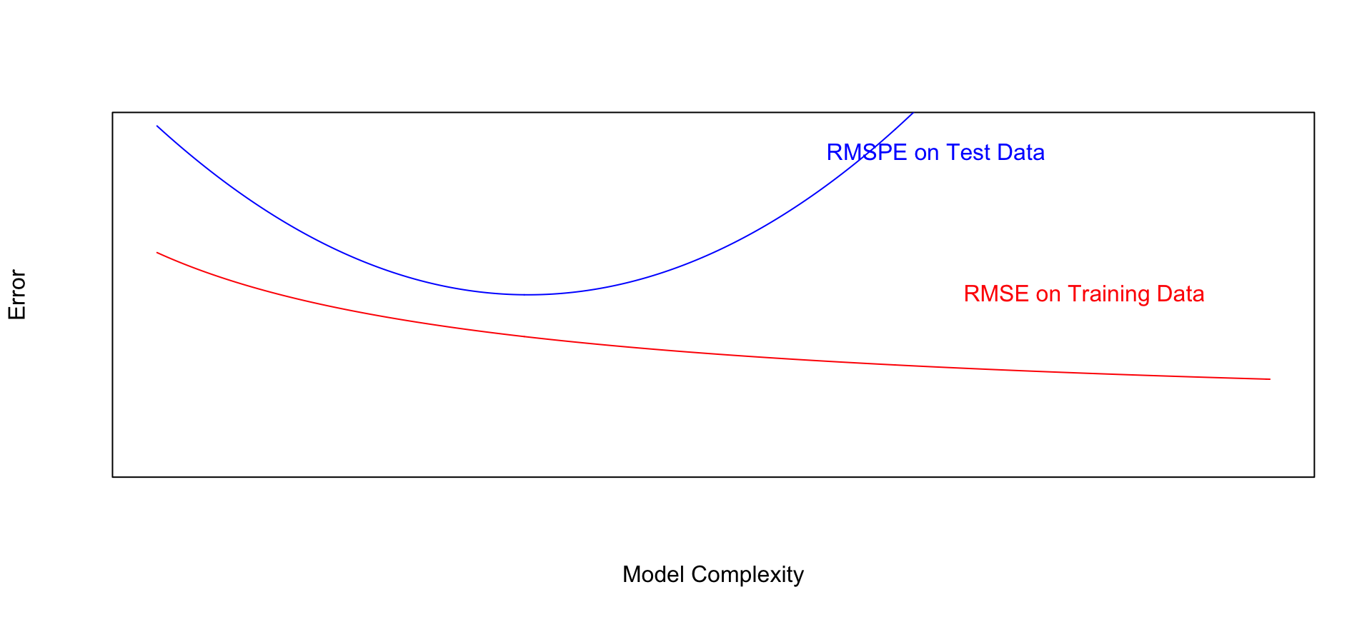
## 9 8 3.350198 2.7990668.1.22 Graph of RMSPE
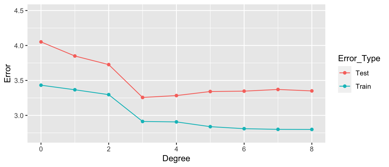
- Training error decreases as model becomes more complex
- Testing error is lowest for the 3rd degree model, then starts to increase again
8.1.23 Third Degree Model Summary
summary(Sim_M3)##
## Call:
## lm(formula = y ~ x + I(x^2) + I(x^3), data = Sampdf)
##
## Residuals:
## Min 1Q Median 3Q Max
## -8.9451 -1.7976 0.1685 1.3988 6.8064
##
## Coefficients:
## Estimate Std. Error t value Pr(>|t|)
## (Intercept) -0.54165 1.26803 -0.427 0.670221
## x 4.16638 1.09405 3.808 0.000247 ***
## I(x^2) -1.20601 0.25186 -4.788 0.00000610 ***
## I(x^3) 0.08419 0.01622 5.191 0.00000117 ***
## ---
## Signif. codes: 0 '***' 0.001 '**' 0.01 '*' 0.05 '.' 0.1 ' ' 1
##
## Residual standard error: 2.973 on 96 degrees of freedom
## Multiple R-squared: 0.2794, Adjusted R-squared: 0.2569
## F-statistic: 12.41 on 3 and 96 DF, p-value: 0.00000063098.1.24 True Data Model
In fact, the data were generated from the model \(y_i = 4.5x - 1.4x^2 + 0.1x^3 + \epsilon_i\), where \(\epsilon_i\sim\mathcal{N}(0,3)\)
8.1.25 True Data Model
In fact, the data were generated from the model \(y_i = 4.5x - 1.4x^2 + 0.1x^3 + \epsilon_i\), where \(\epsilon_i\sim\mathcal{N}(0,3)\)
The yellow curve represents the true expected response curve.
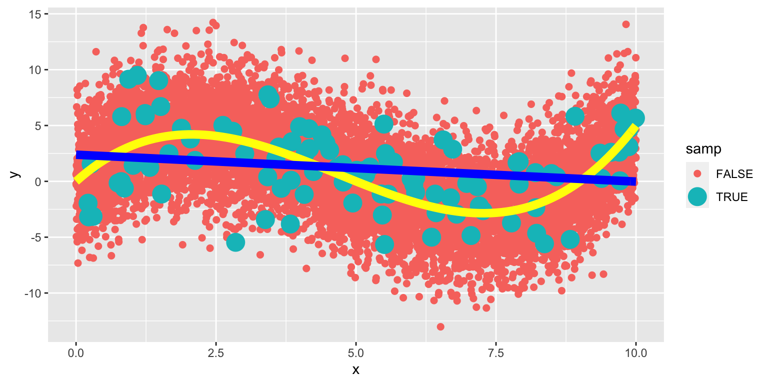
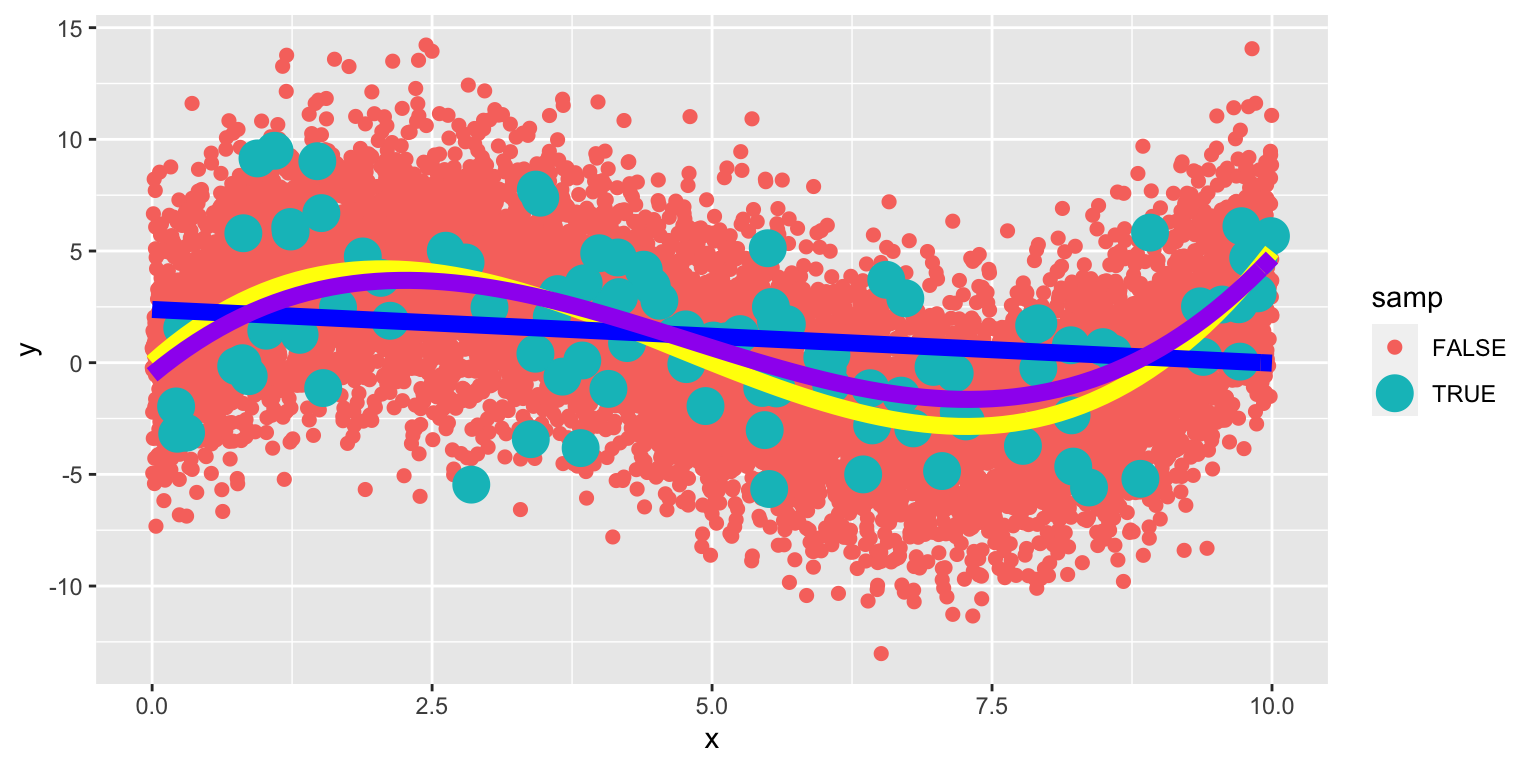
8.1.26 Linear Model on Larger Population
The yellow curve represents the true expected response curve.
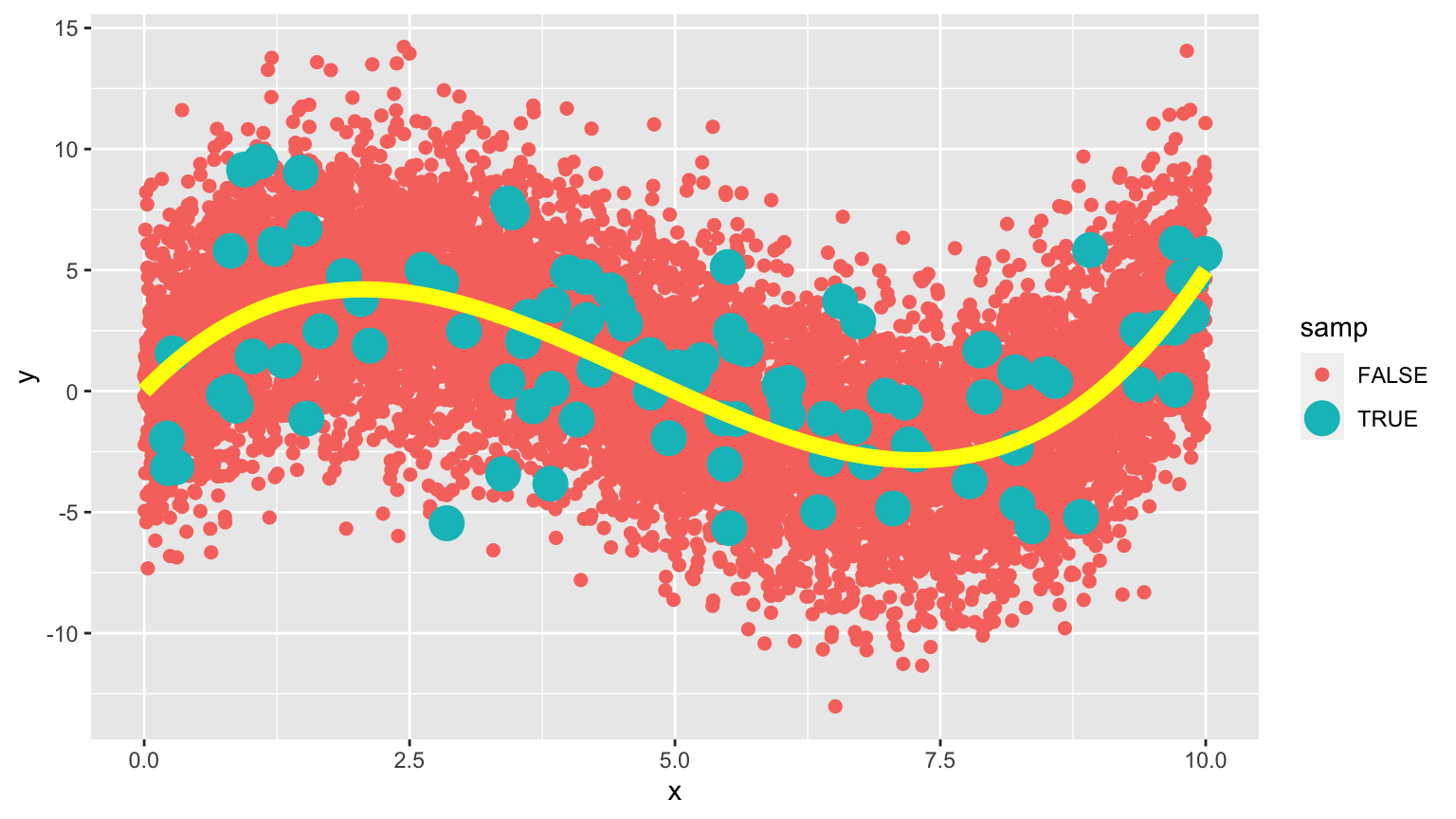
8.1.27 Cubic Model on Larger Population
The yellow curve represents the true expected response curve.
8.1.28 Eighth-Degree Model on Larger Population
The yellow curve represents the true expected response curve.
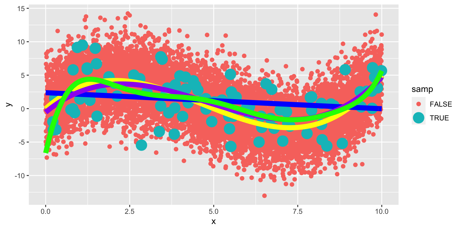
The 8th degree model performs worse than the cubic. The extra terms cause the model to be “too flexible,” and it starts to model random fluctuations (noise) in the training data, that do not capture the true trend for the population. This is called overfitting.
8.1.29 Model Complexity, Training Error, and Test Error
8.2 Variance-Bias Tradeoff
8.2.1 What Contributes to Prediction Error?
Suppose \(Y_i = f(x_i) + \epsilon_i\), where \(\epsilon_i\sim\mathcal{N}(0,\sigma)\).
Let \(\hat{f}\) represent the function of our explanatory variable(s) \(x^*\) used to predict the value of response variable \(y^*\). Thus \(\hat{y}^* = f(x^*)\).
There are three factors that contribute to the expected value of \(\left(y^* - \hat{y}\right)^2 = \left(y^* - \hat{f}(x^*)\right)^2\).
Bias associated with fitting model: Model bias pertains to the difference between the true response function value \(f(x^*)\), and the average value of \(\hat{f}(x^*)\) that would be obtained in the long run over many samples.
- for example, if the true response function \(f\) is cubic, then using a constant, linear, or quadratic model would result in biased predictions for most values of \(x^*\).Variance associated with fitting model: Individual observations in the training data are subject to random sampling variability. The more flexible a model is, the more weight is put on each individual observation increasing the variance associated with the model.
Variability associated with prediction: Even if we knew the true value \(f(x^*)\), which represents the expected value of \(y^*\) given \(x=x^*\), the actual value of \(y^*\) will vary due to random noise (i.e. the \(\epsilon_i\sim\mathcal{N}(0,\sigma)\) term).
8.2.2 Variance and Bias
The third source of variability cannot be controlled or eliminated. The first two, however are things we can control. If we could figure out how to minimize bias while also minimizing variance associated with a prediction, that would be great! But…
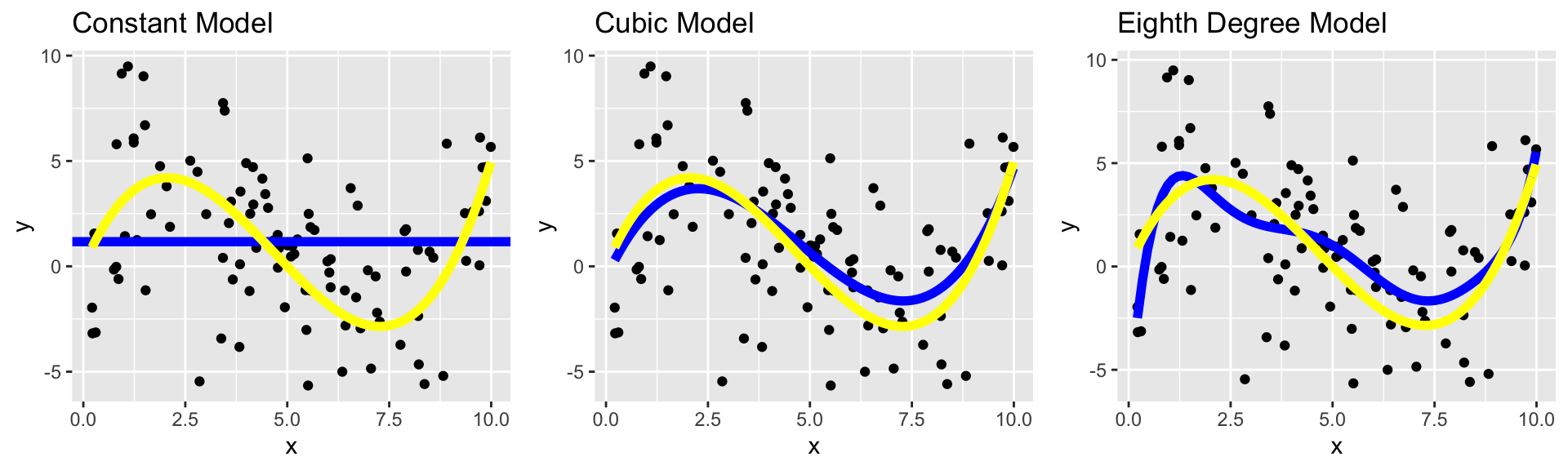
The constant model suffers from high bias. Since it does not include a linear, quadratic, or cubic term, it cannot accurately approximate the true regression function.
The Eighth degree model suffers from high variance. Although it could, in theory, approximate the true regression function correctly, it is too flexible, and is thrown off because of the influence of individual points with high degrees of variability.
8.2.3 Variance-Bias Tradeoff
As model complexity (flexibility) increases, bias decreases. Variance, however, increases.
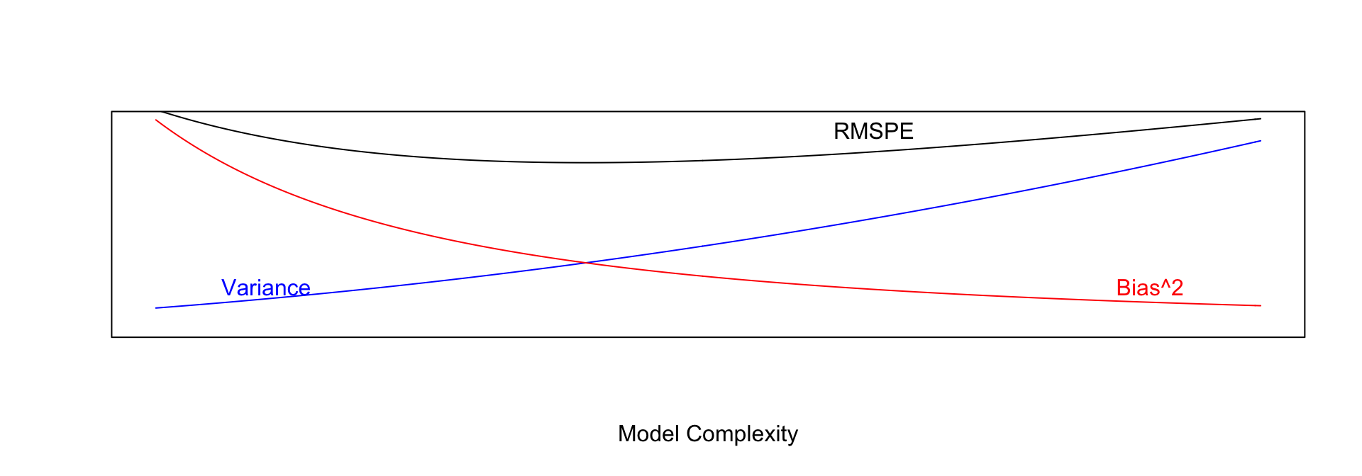
In fact, it can be shown that:
\(\text{Expected RMSPE} = \text{Variance} + \text{Bias}^2\)
Our goal is the find the “sweetspot” where expected RMSPE is minimized.
8.3 Cross-Validation
8.3.1 Cross-Validation (CV)
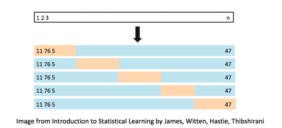
We’ve seen that training error is not an accurate approximation of test error. Instead, we’ll approximate test error, by setting aside a set of the training data, and using it as if it were a test set. This process is called cross-validation, and the set we put aside is called the validation set.
- Partition data into disjoint sets (folds). Approximately 5 folds recommended.
- Build a model using 4 of the 5 folds.
- Use model to predict responses for remaining fold.
- Calculate root mean square error \(RMSPE=\displaystyle\sqrt{\frac{\sum((\hat{y}_i-y_i)^2)}{n'}}\).
- Repeat for each of 5 folds.
- Average RMSPE values across folds.
If computational resources permit, it is often beneficial to perform CV multiple times, using different sets of folds.
8.3.2 Cross-Validation Illustration
8.3.3 Models for Price of New Cars
Consider the following five models for predicting the price of a new car:
M1 <- lm(data=Cars2015, LowPrice~Acc060)
M2 <- lm(data=Cars2015, LowPrice~Acc060 + I(Acc060^2))
M3 <- lm(data=Cars2015, LowPrice~Acc060 + I(Acc060^2) + Size)
M4 <- lm(data=Cars2015, LowPrice~Acc060 + I(Acc060^2) + Size + PageNum)
M5 <- lm(data=Cars2015, LowPrice~Acc060 * I(Acc060^2) * Size)
M6 <- lm(data=Cars2015, LowPrice~Acc060 * I(Acc060^2) * Size * PageNum)
8.3.4 Cross Validation in Cars Dataset
To Use cross validation on the cars dataset, we’ll fit each model to 4 folds (88 cars), while withholding the other 1 fold (22 cars).
We then make predictions on the last fold, and see which model yields the lowest MSPE.
t(Fold)## [,1] [,2] [,3] [,4] [,5] [,6] [,7] [,8] [,9] [,10] [,11] [,12] [,13]
## fold1 76 82 73 14 30 15 109 5 102 92 25 24 6
## fold2 65 80 107 62 8 4 91 75 2 41 99 81 37
## fold3 68 101 108 31 23 59 105 42 35 21 1 84 106
## fold4 50 104 13 52 29 98 66 54 49 110 38 48 63
## fold5 55 22 17 3 10 28 39 51 20 47 69 83 88
## [,14] [,15] [,16] [,17] [,18] [,19] [,20] [,21] [,22]
## fold1 36 16 57 44 72 53 86 94 34
## fold2 74 56 27 90 19 40 61 78 71
## fold3 60 43 77 64 67 100 7 58 87
## fold4 12 103 97 85 95 96 32 45 89
## fold5 9 70 46 11 33 79 26 93 188.3.5 CV Results
Rows show RMSPE, columns show model.
kable(RMSPE)| 11.329817 | 11.460672 | 9.989957 | 10.130743 | 10.808705 | 10.66698 |
| 11.904377 | 12.406512 | 10.998581 | 10.993984 | 13.447907 | 17.27614 |
| 10.044277 | 9.399102 | 8.482429 | 9.167676 | 7.906023 | 13.84186 |
| 9.868489 | 9.081304 | 10.658656 | 10.661173 | 9.435986 | 12.09450 |
| 10.630225 | 9.538196 | 9.178224 | 9.681109 | 8.266503 | 18.80454 |
Mean RMSPE
apply(RMSPE,2,mean)## [1] 10.755437 10.377157 9.861570 10.126937 9.973025 14.5368038.3.6 CV Conclusions
Model 3 achieves the best performance using cross-validation.
This is the model that includes a quadratic function of acceleration time and size.
Including page number, or interactions harms the performance of the model.
We should use model 3 if we want to make predictions on new data.