3 Path analysis

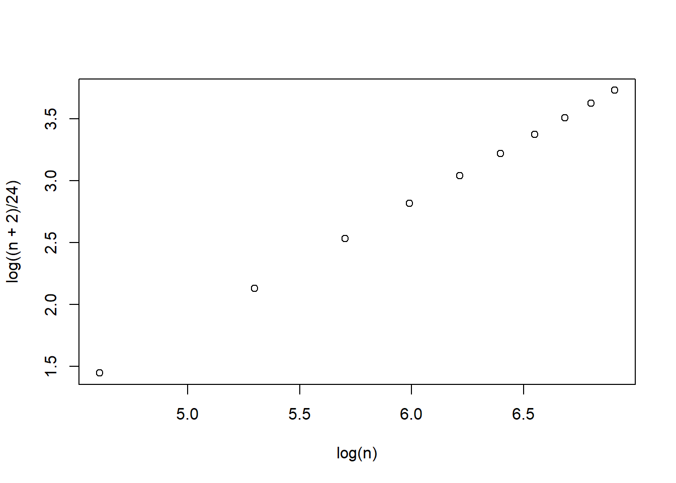
An easy and convenient representation of the relationships among a number of variables is using path diagram, we have saw a lot in past chapters. A path diagram can be viewed as a hypothesised/theory-based model, specifying the structure among variables in interest. We collect data to test whether our sample support the proposed model. Basically, path analysis is the analysis of the “path”.

3.1 Path diagram

Rectangle: observed or manifest variable
Circle: latent variable (i.e. error, factor)
Single-headed arrow: linear relationship between two variables, starts from an independent variable and ends on a dependent variable.
Double-headed arrow: variance of a variable or covariance between two variables.

3.2 What is the difference between multiple regression and path analysis

In path analysis, a variable can be both dependent variable and independent variable at the same time, e.g. mediator, in multiple regression, dependent variable can not be independent variable.
Multiple regression is more restricted in terms of the type of hypothesis it can test. We can only test whether a independent variable can effectively predict dependent variable while controlling other predictors; whereas path analysis can do more than that, e.g. mediation mechanism.

3.3 Effects Decomposition

When doing path analysis, we impose a theoretical structure upon our variables and derive \(\boldsymbol{\Sigma}(\boldsymbol{\theta})\). In \(\boldsymbol{\Sigma}(\boldsymbol{\theta})\), all the variances/correlations between one independent variable and one dependent variable can be partitioned into a summation of different parts using model parameters. This is called effects decomposition. There are four types of possible resulting effects.

3.3.1 Four types of effects

Causal effect (most important)

Direct effect: a direct effect is represented by a single causal arrow from a independent variable to a dependent variable, i.e. \(x\) leads to \(y\), the change in \(x\) will “cause” a change in \(y\);
Indirect effect: an indirect effect is represented by two or more spliced causal arrows between an independent variable and a dependent variable, i.e. \(x\) leads to \(m\), \(m\) leads to \(y\), the causal effect of \(x\) on \(y\) is transmitted via \(m\);

Non-causal effect

Undecomposed effect: when there exists causal effect between an independent variable and a dependent variable, the causal effect accounts for part of the covariance/correlation between these two variables, the rest part of their covariance/correlation is undecomposed effect because it can not be decomposed clearly. This is usually because there is another independent variable that is in the same regression model but correlated with the very independent variable, we do not know which independent variable should be responsible for the leftover covariance/correlation. i.e. \(x_1\) and \(x_2\) are two predictors of \(y\), the change in \(x_1\) can spread into \(x_2\) (because correlated), and the change in \(x_2\) lead to change in \(y\);
Spurious covariance/correlation: the part of covariance/correlation between two dependent variables that roots in having same independent variable or correlated independent variables, i.e. \(x\) is the predictor of both \(y_1\) and \(y_2\), the change in \(x\) will lead to change in \(y_1\) and \(y_2\), making \(y_1\) and \(y_2\) seemingly correlated.

3.3.2 Effects decomposition via tracing diagram and \(\boldsymbol{\Sigma(\theta)}\)

Let’s look at an example, we have four variable:

SES: social economic status
IQ: intelligence quotient
nACH: need for achievement
GPA: grade-point average

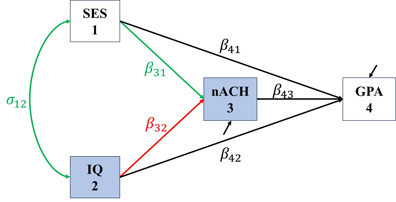
We specify the relationship among this four variables as

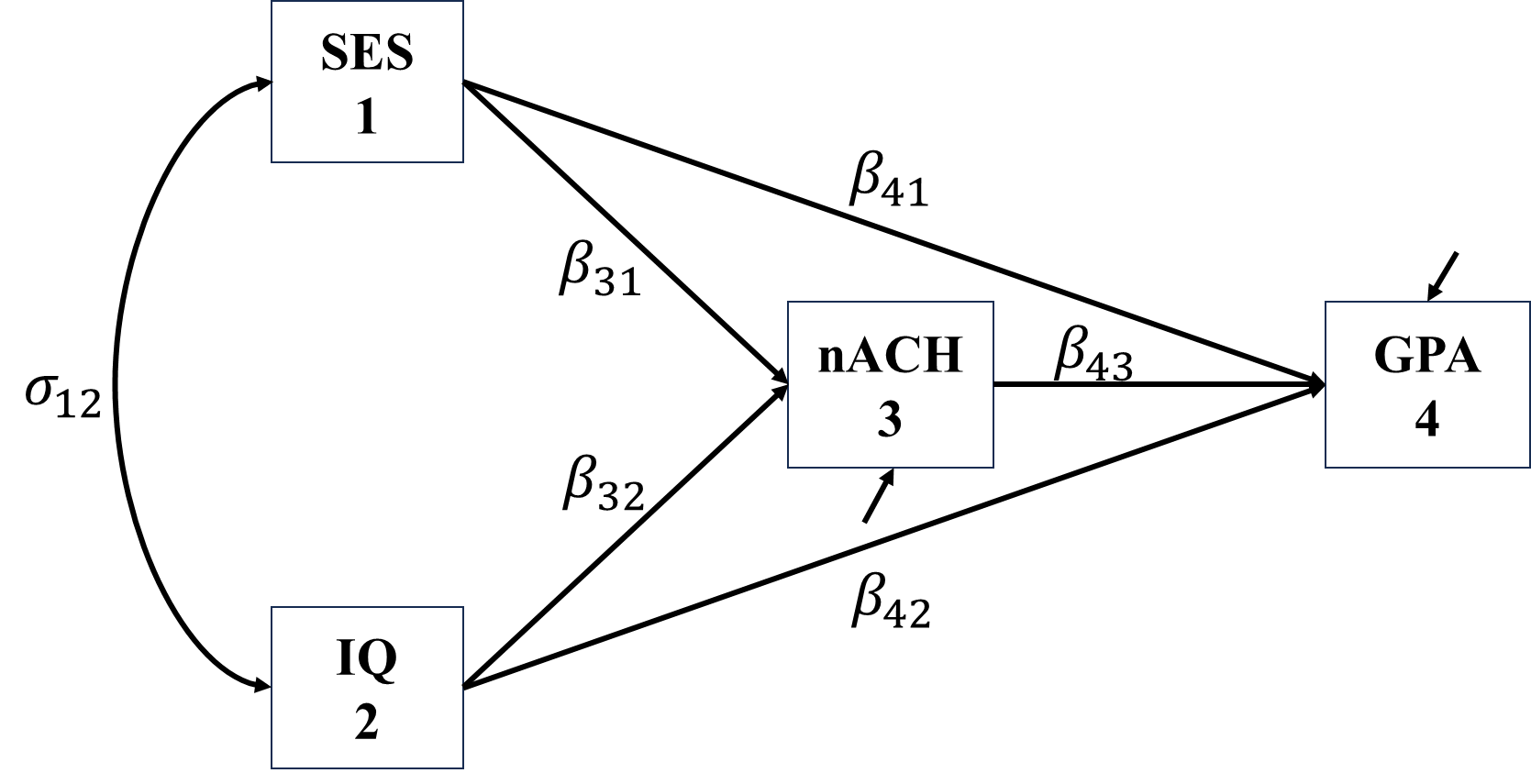
The corresponding regressions are \[\begin{align*} nACH&=\beta_{31}SES+\beta_{32}IQ+\epsilon_{nACH}\\ GPA&=\beta_{41}SES+\beta_{42}IQ+\beta_{43}nACH+\epsilon_{GPA}. \end{align*}\] The resultant \(\boldsymbol{\Sigma(\theta)}\) is \[\begin{align*} \bSigma(\bs{\theta})=\begin{bmatrix} \sigma_{SES}^2 & \sigma_{SES,IQ} & \sigma_{SES,nACH} & \sigma_{SES,GPA} \\ \sigma_{IQ,SES} & \sigma_{IQ}^2 & \sigma_{IQ,nACH} & \sigma_{IQ,GPA}\\ \sigma_{nACH,SES} & \sigma_{nACH,IQ} & \sigma_{nACH}^2 & \sigma_{nACH,GPA}\\ \sigma_{GPA,SES} & \sigma_{GPA,IQ} & \sigma_{GPA,nACH} & \sigma_{GPA}^2 \end{bmatrix}. \end{align*}\]

In the following figures, red represents direct effects, blue represent indirect effects, green represents undecomposited effects, and grey represents spurious covariance/correlation.

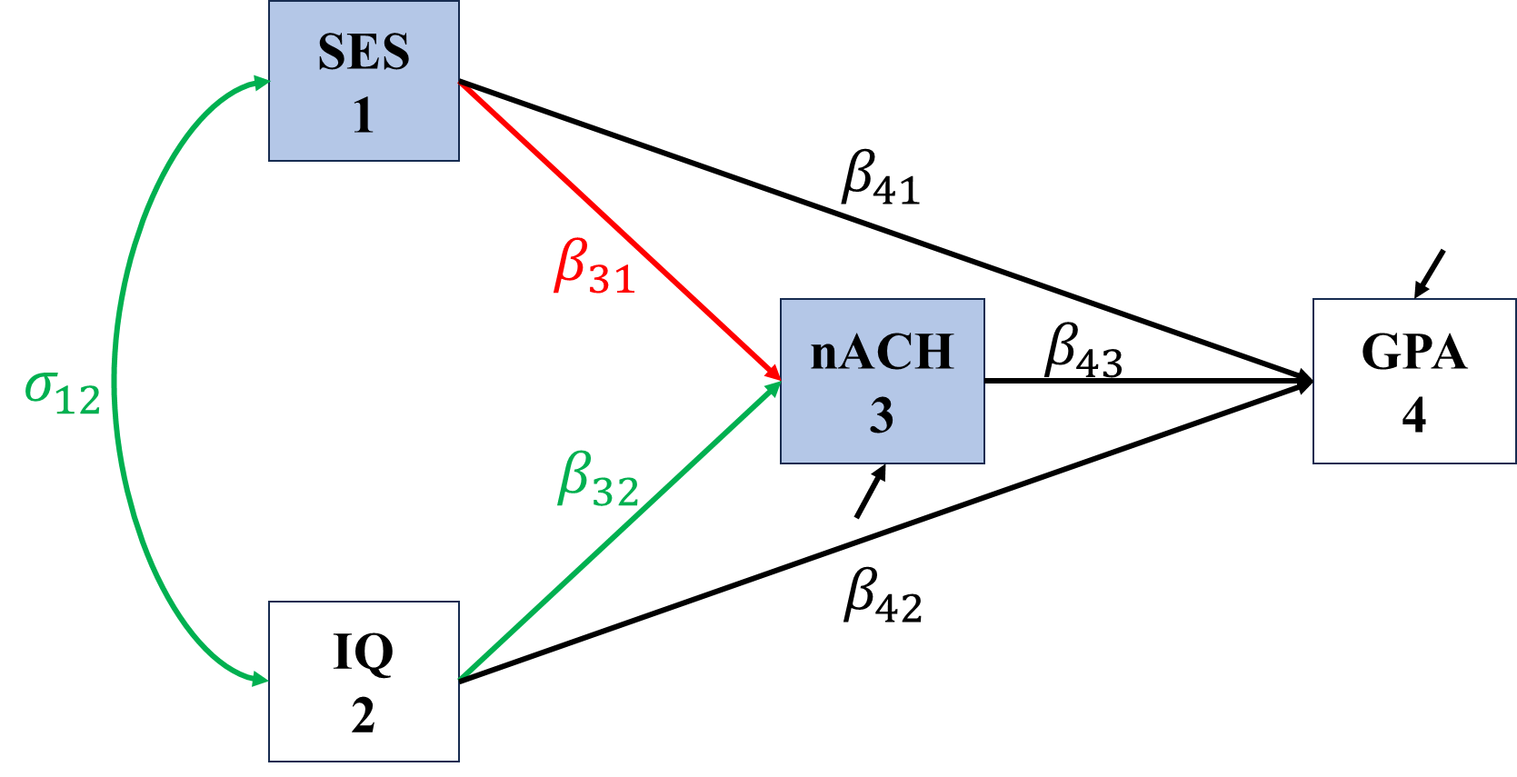
The decomposition of \(\sigma_{SES,nACH}\)

\[\begin{align*} \sigma_{SES,nACH}&=\Cov(SES,\beta_{31}SES+\beta_{32}IQ+\epsilon_{nACH})\\ &=\color{red}\beta_{31}\sigma_{SES}^2+\color{green}\beta_{32}\sigma_{SES,IQ}, \end{align*}\]

The decomposition of \(\sigma_{IQ,nACH}\)

\[\begin{align*} \sigma_{IQ,nACH}&=\Cov(IQ,\beta_{31}SES+\beta_{32}IQ+\epsilon_{nACH})\\ &=\color{red}\beta_{32}\sigma_{IQ}^2+\color{green}\beta_{31}\sigma_{IQ,SES} \end{align*}\]

The decomposition of \(\sigma_{SES,GPA}\)

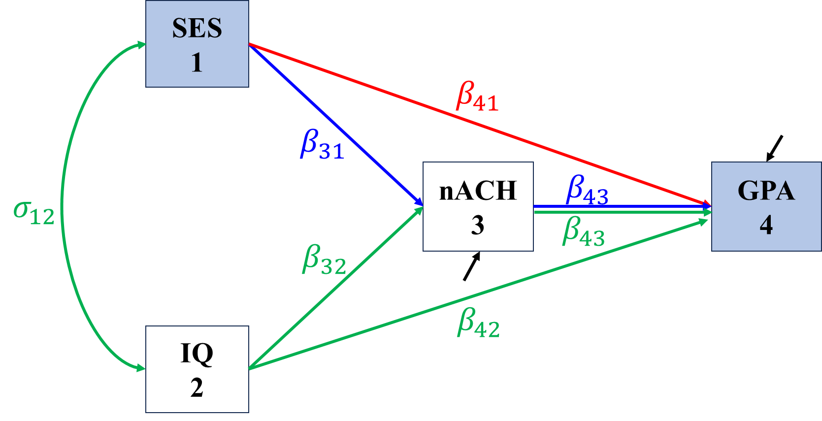
\[\begin{align*} \sigma_{SES,GPA}&=\Cov(SES,\beta_{41}SES+\beta_{42}IQ+\beta_{43}nACH+\epsilon_{GPA})\\ &=\beta_{41}\sigma_{SES}^2+\beta_{42}\sigma_{SES,IQ}+\beta_{43}\sigma_{SES,nACH}\\ &=\color{red}\beta_{41}\sigma_{SES}^2+\color{blue}\beta_{43}\beta_{31}\sigma_{SES}^2+\color{green}\beta_{42}\sigma_{SES,IQ}+\beta_{43}\beta_{32}\sigma_{SES,IQ}. \end{align*}\]

The decomposition of \(\sigma_{IQ,GPA}\)

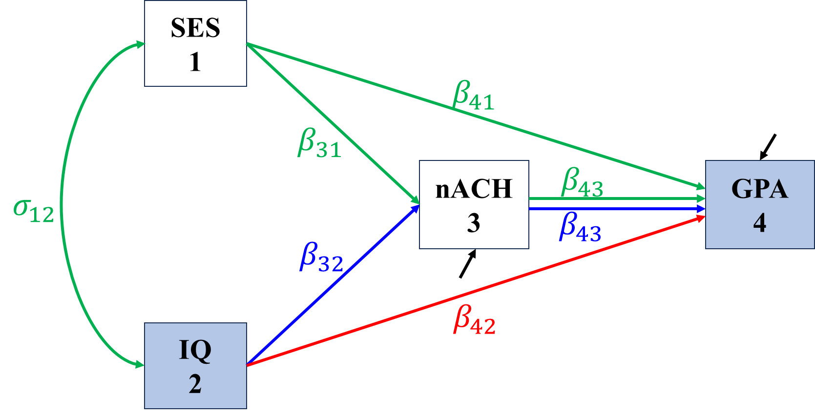
\[\begin{align*} \sigma_{IQ,GPA}&=\Cov(IQ,\beta_{41}SES+\beta_{42}IQ+\beta_{43}nACH+\epsilon_{GPA})\\ &=\beta_{41}\sigma_{IQ,SES}+\beta_{42}\sigma_{IQ}^2+\beta_{43}\sigma_{IQ,nACH}\\ &=\color{red}\beta_{42}\sigma_{IQ}^2+\color{blue}\beta_{43}\beta_{32}\sigma_{IQ}^2+\color{green}\beta_{41}\sigma_{IQ,SES}+\beta_{43}\beta_{31}\sigma_{IQ,SES}. \end{align*}\]

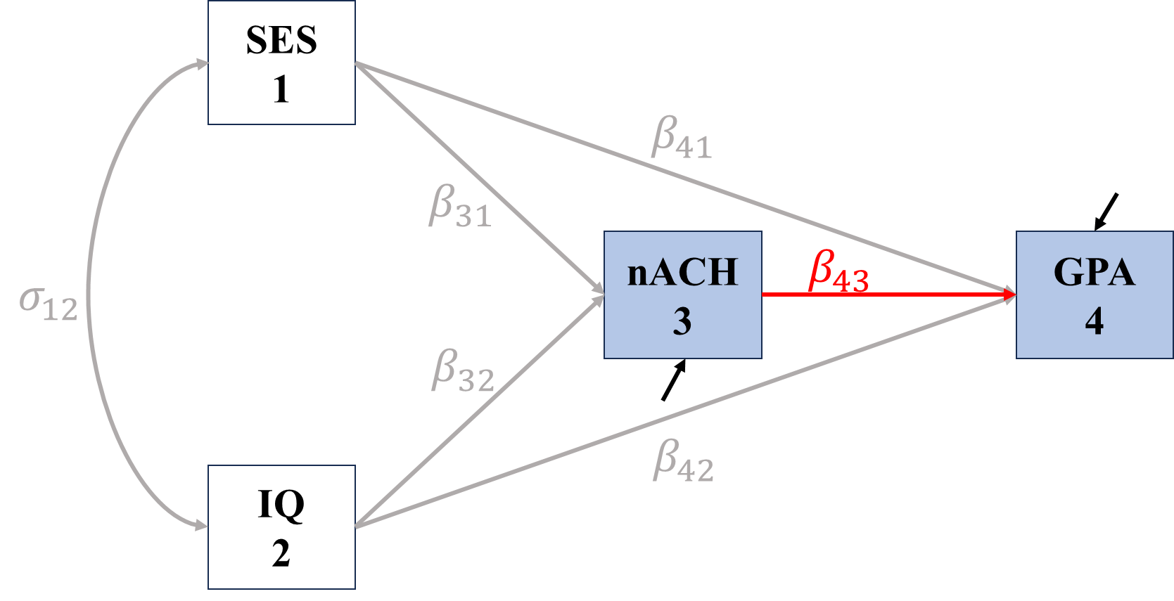
The decomposition of \(\sigma_{nACH,GPA}\)

\[\begin{align*} \sigma_{nACH,GPA}&=\Cov(nACH, \beta_{41}SES+\beta_{42}IQ+\beta_{43}nACH+\epsilon_{GPA})\\ &=\beta_{41}\sigma_{nACH,SES}+\beta_{42}\sigma_{nACH,IQ}+\beta_{43}\sigma_{nACH}^2\\ &=\color{red}\beta_{43}\sigma_{nACH}^2+\\ &\color{Grey}\quad\text{ }\beta_{41}\beta_{31}\sigma_{SES}^2+\beta_{41}\beta_{32}\sigma_{SES,IQ}+\\ &\color{Grey}\quad\text{ }\beta_{42}\beta_{32}\sigma_{IQ}^2+\beta_{42}\beta_{31}\sigma_{IQ,SES} \end{align*}\]

By standardize all variables, the variance terms becomes 1 and disappear, the covariance terms become correlations, and the regression coefficients become standardized ones, we have

\[\begin{align*} \rho_{SES,nACH}&=\color{red}\beta_{31}+\color{green}\beta_{32}\rho_{SES,IQ}\\ \rho_{IQ,nACH}&=\color{red}\beta_{32}+\color{green}\beta_{31}\rho_{IQ,SES}\\ \rho_{SES,GPA}&=\color{red}\beta_{41}+\color{blue}\beta_{43}\beta_{31}+\color{green}\beta_{42}\rho_{SES,IQ}+\beta_{43}\beta_{32}\rho_{SES,IQ}\\ \rho_{IQ,GPA}&=\color{red}\beta_{42}+\color{blue}\beta_{43}\beta_{32}+\color{green}\beta_{41}\rho_{IQ,SES}+\beta_{43}\beta_{31}\rho_{IQ,SES}\\ \rho_{nACH,GPA}&=\color{red}\beta_{43}+\color{Grey}\beta_{41}\beta_{31}+\beta_{42}\beta_{32}+\beta_{41}\beta_{32}\rho_{SES,IQ}+\beta_{42}\beta_{31}\rho_{IQ,SES} \end{align*}\]

Once the estimated parameters are available, it is very easy to manually conduct the effects decomposition of given two variables. For example, with the estimated paths below, the indirect effect between \(SES\) and \(GPA\) is \(0.398\times0.416\).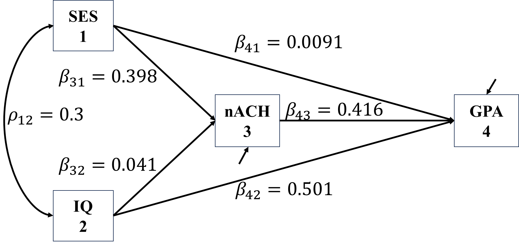

3.3.3 Homework

ex3.11

Decompose \(r_{x1y3}\);

3.4 Modeling process

After specifying a theoretical structure, the next step of SEM analysis (including path analysis), is modeling, i.e. collecting data and evaluating model. When dealing with multiple variables, it is very likely that we can have a group of competing models, we do not know which one is the best, we have to perform model evaluation in roughly two steps:

model estimation: obtain the optimal estimates of unknown parameters and model-data fit for these model;
model comparison: compare the model-data fit to find the best model.

3.4.1 Model estimation

3.4.1.1 Four basic matrices in SEM

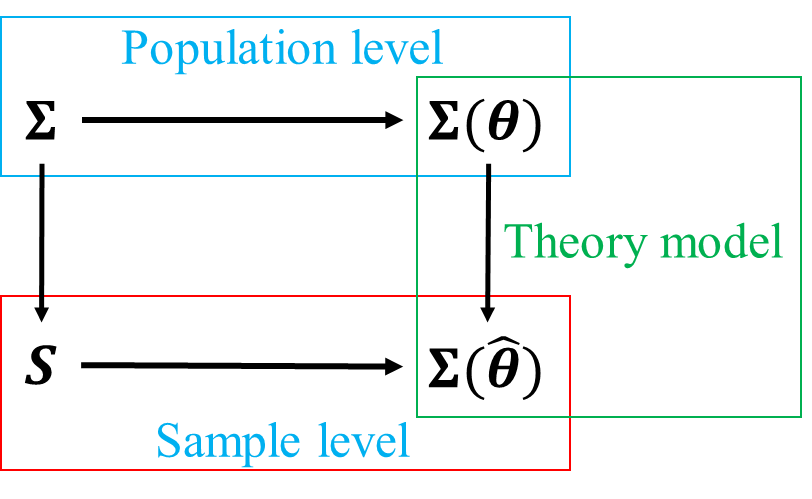
At population level, when studying a set of mutually correlated variables, the covariance matrix of these variables is \(\boldsymbol{\Sigma}\). If we imposed a structure with unknown parameters \(\boldsymbol{\theta}\) upon these group of variables, we can derive the model-implied covariance matrix \(\boldsymbol{\Sigma}(\boldsymbol{\theta})\). If the structure we specified was true, i.e. correctly represent the relationship among variables in interest, then \(\boldsymbol{\Sigma}=\boldsymbol{\Sigma}(\boldsymbol{\theta})\).

At sample level, the sample estimator of \(\boldsymbol{\Sigma}\) is sample covariance matrix \(\boldsymbol{S}\), the sample estimator of \(\boldsymbol{\Sigma}(\boldsymbol{\theta})\) is \(\boldsymbol{\Sigma}(\hat{\boldsymbol{\theta}})\). If we specified the true model, \(\boldsymbol{S}\) should be closely approximated by \(\boldsymbol{\Sigma}(\hat{\boldsymbol{\theta}})\), but due to sampling error, they won’t be exactly the same.

If we misspecified a wrong model, then the discrepancy between \(\boldsymbol{\Sigma}\) and \(\boldsymbol{\Sigma}(\boldsymbol{\theta})\) will undoubtedly increase, so will that between \(\boldsymbol{S}\) and \(\boldsymbol{\Sigma}(\hat{\boldsymbol{\theta}})\). Therefore, when performing model evaluation, we are effectively trying to find the best model with \(\hat{\boldsymbol{\theta}}\) that can minimize the discrepancy between \(\boldsymbol{S} - \boldsymbol{\Sigma}(\hat{\boldsymbol{\theta}})\).

3.4.1.2 Discrepancy function

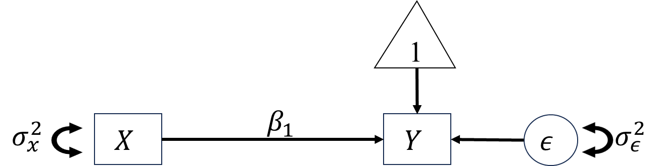
The purpose of model estimation is to find the best sample estimates for the unknown parameters in a given model. The “best” is achieved by minimize the discrepancy using sample. For example (this example is taken from the lecture note of SEM class taught by Professor Zhang Zhiyong at University of Notre Dame), we have two random variables \(x\) and \(y\) with

\[\begin{align} \boldsymbol{S}=\begin{bmatrix} 2 & 1 \\ 1 & 2 \end{bmatrix} \end{align}\]

We assume the true relationship between \(x\) and \(y\) is \(y=\beta x+\epsilon\), thus we have

\[\begin{align} \boldsymbol{\Sigma}(\boldsymbol{\theta})= \begin{bmatrix} \sigma^2_x & \beta\sigma^2_x \\ \beta\sigma^2_x & \beta^2\sigma^2_x+\sigma^2_\epsilon \end{bmatrix}, \end{align}\]

where the unknown parameters are \(\beta\), \(\sigma^2_x\), and \(\sigma^2_\epsilon\). We can try different sets of \(\hat{\theta}\) to see how \(\boldsymbol{S} - \boldsymbol{\Sigma}(\hat{\boldsymbol{\theta}})\) differ. When \(\hat{\bs{\theta}}_1=(0,1,1)\),

\[\begin{align} \boldsymbol{\Sigma}(\hat{\boldsymbol{\theta}}_1)= \begin{bmatrix} 1 & 0 \\ 0 & 1 \end{bmatrix}, \end{align}\]

then

\[\begin{align} \boldsymbol{S} - \boldsymbol{\Sigma}(\hat{\boldsymbol{\theta}}_1)= \begin{bmatrix} 1 & 1 \\ 1 & 1 \end{bmatrix}. \end{align}\]

When \(\hat{\bs{\theta}}_2=(1,1,1)\),

\[\begin{align} \boldsymbol{\Sigma}(\hat{\boldsymbol{\theta}}_2)= \begin{bmatrix} 1 & 1 \\ 1 & 2 \end{bmatrix}, \end{align}\]

and

\[\begin{align} \boldsymbol{S} - \boldsymbol{\Sigma}(\hat{\boldsymbol{\theta}}_2)= \begin{bmatrix} 1 & 0 \\ 0 & 0 \end{bmatrix}. \end{align}\]

It is clear that for this given model, \(\hat{\boldsymbol{\theta}}_2\) is better, but we do not know whether \(\hat{\boldsymbol{\theta}}_2\) is the best sample estimate of \(\bs{\theta}\). We need to quantify the difference between two matrices with identical size and an algorithm to minimize the difference to find the best \(\hat{\boldsymbol{\theta}}\).

Noted that, \(\boldsymbol{S} - \boldsymbol{\Sigma}(\hat{\boldsymbol{\theta}})\) is actually a matrix function of \(\hat{\boldsymbol{\theta}}\), called discrepancy function \(\boldsymbol{F}\). Minimizing a matrix function quickly becomes unmanageable as the size of matrix function increase. To that end, we usually summarize the difference between \(\boldsymbol{S}\) and \(\boldsymbol{\Sigma}(\hat{\boldsymbol{\theta}})\) as a scalar discrepancy function \(F\), different estimation methods only differ in the way they summarize.

3.4.1.3 Common estimation methods (skimming)

Ordinal least square (OLS)

\(F_{OLS}(\boldsymbol{\theta})=[\boldsymbol{s}-\boldsymbol{\sigma}(\theta)]'[\boldsymbol{s}-\boldsymbol{\sigma}(\theta)],\)

where \(\boldsymbol{s}\) and \(\boldsymbol{\sigma}(\theta)\) are the \(p(p+1)/2\) unique elements from \(\boldsymbol{S}\) and \(\boldsymbol{\Sigma}\), respectively.

Multivariate normal distribution maximum likelihood (NML)

\(F_{NML}=\log|\boldsymbol{\Sigma}(\boldsymbol{\theta})|+\text{tr}(\boldsymbol{S}\boldsymbol{\Sigma}^{-1}(\boldsymbol{\theta}))-\log|\boldsymbol{S}|-p.\)

NML is usually the default estimation method in most SEM software. Note that, \((n-1)F_{NML}=-2\log\lambda=T\).

3.4.2 Model fit

After fitting a specified model to data, we answer the question “how good is our model” by model-data fit. Model fit indices abound, most of them are directly based on likelihood ratio test (LRT).

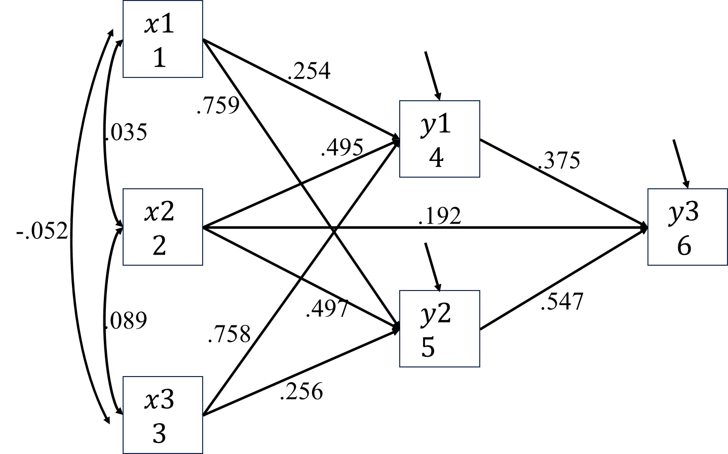
3.4.2.1 The best model and the worst model

In SEM, the best model we can fit to data is the \(\boldsymbol{\Sigma}(\boldsymbol{\theta})=\boldsymbol{S}\), that is the saturated model/unrestricted model/just-identified model. It is worth noting that in path analysis, unrestricted model means all possible paths are allowed, saturated because no extra parameter can be added to the existing model, \(df=0\). Following is an example of saturated model.

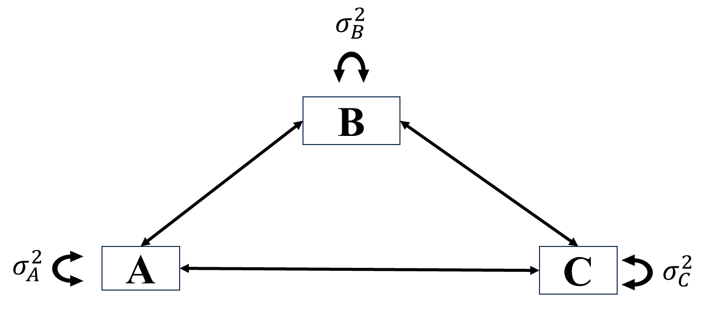
The worst model we can fit to data is the baseline model/null model. In this model, all \(p\) variables are assumed to be independent to each other, thus the resulting \(\boldsymbol{\Sigma}(\boldsymbol{\theta})=I_P\).

3.4.2.2 Incremental measure of fit

In SEM, \(\text{T}=(n-1)F_{\text{ML}}\) is the LRT test statistics of tested model (\(H_0\) model), it asymptotically follows \(\chi^2\) distribution with \(df=p(p+1)/2-q\), where \(q\) is the number of parameters.

\[\begin{align*} \text{Comparative Fit Index, CFI}=1-\frac{\max(\text{T}-df,0)}{\max(\text{T}_0-df_0,\text{T}-df)}, \end{align*}\] where \(\text{T}_0\) is the resulting test statistics of LRT if we fit null model to data, and \(df_0=p(p+1)/2\). CFI measures the extent that fitted model improves compared with the null model. It is restricted between 0 and 1.

\[\begin{align*} \text{Tucker Lewis Index, TLI/Non-normed Fit Index, NNFI}=1-\frac{df_0}{df}\left(\frac{\text{T}-df}{\text{T}_0-df_0}\right). \end{align*}\] TLI adds penalty for complex model, thus tend to endorse model with less parameters, Note that, CFI and TLI should be very close to each other. If the CFI is less than one, then the CFI is always greater than the TLI, only one of the two should be reported to avoid redundancy. But TLI could exceed 1 under certain condition, if so, it is capped at 1 in most SEM software, except for Mplus.

For CFI and TLI:

\(>0.95\) indicates good model-data fit
\(>0.9\) indicates acceptable model-data fit

\[\begin{align*} \text{Root Mean Square Error of Approximation, RMSEA}=\sqrt{\frac{\text{T}-df}{df(n-1)}}. \end{align*}\] RMSEA measures the average model misfit per \(df\). It is always positive. Just like TLI, RMSEA tends to endorse small-size model. There is greater sampling error for small \(df\) and low \(n\) models, especially for the former. Thus, models with small \(df\) and low \(n\) can have artificially large values of the RMSEA. For instance, a \(\text{T}\) of 2.098 (a value not statistically significant), with a \(df\) of 1 and \(n\) of 70 yields an RMSEA of 0.126. For this reason Kenny & Kaniskan (2014) argue to not even compute the RMSEA for low \(df\) models.

A confidence interval can be computed for the RMSEA. Its formula is based on the non-central \(\chi^2\) distribution and usually the 90% interval is used. Ideally the lower value of the 90% confidence interval includes or is very near zero (or no worse than 0.05) and the upper value is not very large, i.e., less than 0.08 or perhaps a 0.10. The width of the confidence interval can be very informative about the precision in the estimate of the RMSEA.

\(\text{RMSEA}\leq 0.05\) indicates a close fit of a model
\(\text{RMSEA}\leq 0.08\) indicates a reasonable model
\(\text{RMSEA}>1\) indicates a bad model

Note that CFI, TLI and RMSEA treat a \(\text{T}=df\) as the best possible model.

\[\begin{align*} \text{Standardized Root Mean Square Residual, SRMR}=\sqrt{\frac{2\sum_{i=1}^p\sum_{j=1}^{i}\left[\frac{s_{ij}-\hat{\sigma}_{ij}}{s_{ii}s_{jj}}\right]^2}{p(p+1)}}. \end{align*}\]

The SRMR is an absolute measure of fit and is defined as the standardized difference between the observed correlation and the predicted correlation. It is a positively biased measure and that bias is greater for small \(N\) and for low \(df\) studies. Because the SRMR is an absolute measure of fit, a value of zero indicates perfect fit. The SRMR has no penalty for model complexity. A value less than .08 is generally considered a good fit (Hu & Bentler, 1999).

3.4.2.3 Comparative measure of fit

Flowing are 3 commonly used comparative measure of fit, Akaike Information Criterion (AIC), Bayesian Information Criterion (BIC), and sample-size adjusted BIC (SABIC).

\[\begin{align*} \text{AIC}&=\text{T}+2q\\ \text{BIC}&=\text{T}+\log(n)q\\ \text{SABIC}&=\text{T}+\log(\frac{n+2}{24})q. \end{align*}\] Because AIC and BIC have no fixed scale, no cut-off value is available.

Lower values of AIC indicate a better fit and so the model with the lowest AIC is the best fitting model. There are somewhat different formulas given for the AIC in the literature, but those differences are not really meaningful as it is the difference in AIC that really matters. The AIC makes the researcher pay a penalty of two for every parameter that is estimated.

BIC increases the penalty as sample size increases. The BIC places a high value on parsimony. The SABIC or SABIC like the BIC places a penalty for adding parameters based on sample size, but not as high a penalty as the BIC.

n <- seq(100, 1000, 100)
plot(log(n), log((n + 2)/24))

3.4.3 Model comparison

In SEM, there are two types of model comparison:

nested model comparison,
unnested model comparison,

Nested model comparison is usually conducted using LRT-based \(\chi^2\) difference test.

A model can be seen as a special case of another by imposing constraints (force to be 0) on parameters. If the model fit of a complex model was good, then constraints can be set to test the resulting simpler model.

\[\Delta_{\text{T}}=\text{T}_{\text{simpler}}-\text{T}_{\text{larger}}\] If \(\Delta_{\text{T}}\) is significant, then the constraints are not appropriate. Otherwise, the simpler model can be used.

Unnested model comparison is usually conducted using fit indices (i.e., 1-factor model vs 2-factor model).

It is usually recommended to report multiple fit indices when comparing models (nested and non-nested), so that we can have more information. But the problem is that fit indices can disagree with each other and we do not know which one is right.

Lai’s paper

3.4.4 JARS Reporting Standards

Some recommendations related to what we just learned:

State the software (including version) used in the analysis. Also state the estimation method used and justify its use (i.e., whether its assumptions are supported by the data, if methods assuming multivariate normality was used, report statistics that measure univariate or multivariate skewness and kurtosis that support the assumption of normal distributions, otherwise state the strategy used to address nonnormality, such as use of a different estimation method that does not assume normality or use of normalizing transformations of the scores).
Disclose any default criteria in the software, such as the maximum number of iterations or level of tolerance, that were adjusted in order to achieve a converged and admissible solution.
Report fit statistics or indices about global (omnibus) fit interpreted using criteria justified by citation of most recent evidence-based recommendations for all models to be interpreted.
State the strategy or criteria used to select one model over another if alternative models were compared. Report results of difference tests for comparisons between alternative models.
Indicate whether one or more interpreted models was a product of respecification. If so, then describe the method used to search for misspecified parameters. State which parameters were fixed or freed to produce the interpreted model. Also provide a theoretical or conceptual rationale for parameters that were fixed or freed after specification searching.
Report both unstandardized and standardized estimates for all estimated parameters.