2  The key concept behind SEM: model-implied covariance matrix $\mathbf{\Sigma }\mathbf{(}\mathit{\theta }\mathbf{)}$

In the following sections within this chapter, we will illustrate the key concept of SEM by comparing SEM with conventional linear regression in a typical multiple regression scenario.

2.1 No mean structure

Because in SEM analysis, we study the relationship among variables by analyzing covariance/correlation. However, the magnitude of covariance between two given variables remains unchanged if we modified their means. We, therefore assume the means of all variables are zero, the resulting structure of interest is called no mean structure. If not this case, one can achieve zero means by centering or standardize data. This is true in most cases, (see Chapter 5 for more information). Analysis on covariance structure without considering means is often called covariance analysis.

2.2 $\mathbf{\Sigma }\mathbf{(}\mathit{\theta }\mathbf{)}$

If we are interested in the relationship between two variables, we normally use covariance/correlation (Person product-moment correlation coefficient) to quantify it. In doing so, we assume these two variables are random variables (more specifically, bivariate normally distributed).

However, in multiple regression, we have one dependent variable, and a set of predictors, $$y_i={\beta }_1{x}_{1i}+\cdots +{\beta }_p{x}_{pi}+{ϵ}_i,$$ where $x_1,\dots ,x_p$ are all fixed values, that is, we treat them as variables, but not random variables. This is so called the multiple regression with fixed $x$. The only random variables in multiple regression with fixed $x$ are $\mathit{y}$ and $\mathit{ϵ}$, where the randomness of $\mathit{y}$ is arguably inherited from $\mathit{ϵ}$. Therefore, theoretically, we are not allowed to quantify the relationship among $x$s and $y$ using either covariance or correlation.

But in SEM, we treat all $x$s and $y$s (yes, we can have more than 1 $y$ in SEM) as random variables. If $x_1$, $\cdots$, $x_p$ are random variables, the above model becomes multiple regression with random $x$ (unless stated otherwise, multiple regression in this book refers to multiple regression with random $x$s), and now we can discuss the relationships among all variables using their covariances. The resultant covariance matrix is $$\begin{array}{r}\mathrm{Cov}(x_1,\cdots ,x_p,y)=\left[\begin{array}{ccc}{\sigma }_{x_1}^2& \cdots & {\sigma }_{x_{1}y}\\ ⋮& & ⋮\\ {\sigma }_{y{x}_1}& \cdots & {\sigma }_y^2\end{array}\right].\end{array}$$ Because we are expressing the relationship among all variables in terms of a multiple regression model, therefore we can use the selected model to re-express the covariance matrix above, and derive a model-implied covariance matrix $\mathbf{\Sigma }\mathbf{(}\mathit{\theta }\mathbf{)}$, where $\mathit{\theta }$ is a vector hosting all unknown model parameters, representing the model specified. For example, for a multiple regression with 2 predictors $x_1$ and $x_2$, $\mathbf{\Sigma }\mathbf{(}\mathit{\theta }\mathbf{)}$ is $$\begin{array}{r}\left[\begin{array}{ccc}{\sigma }_{x_1}^2& {\sigma }_{x_1{x}_2}& {\sigma }_{x_{1}y}\\ {\sigma }_{x_2{x}_1}& {\sigma }_{x_2}^2& {\sigma }_{x_{2}y}\\ {\sigma }_{y{x}_1}& {\sigma }_{y{x}_2}& {\sigma }_y^2\end{array}\right],\end{array}$$ where $$\begin{array}{rl}{\sigma }_{x_{1}y}& =\mathrm{Cov}(x_1,{\beta }_1{x}_1+{\beta }_2{x}_2+ϵ)\\ & ={\beta }_1{\sigma }_{x_1}^2+{\beta }_2{\sigma }_{x_1{x}_2},\end{array}$$ $$\begin{array}{rl}{\sigma }_{x_{2}y}& =\mathrm{Cov}(x_2,{\beta }_1{x}_1+{\beta }_2{x}_2+ϵ)\\ & ={\beta }_1{\sigma }_{x_1{x}_2}+{\beta }_2{\sigma }_{x_2}^2,\end{array}$$ $$\begin{array}{rl}{\sigma }_y^2& =\mathrm{Cov}({\beta }_1{x}_1+{\beta }_2{x}_2+ϵ,{\beta }_1{x}_1+{\beta }_2{x}_2+ϵ)\\ & ={\beta }_1^2{\sigma }_{x_1}^2+{\beta }_2^2{\sigma }_{x_2}^2+2{\beta }_1{\beta }_2{\sigma }_{x_1{x}_2}+{\sigma }_{ϵ}^2.\end{array}$$ What we have now is the model implied covariance structure of $y={\beta }_1{x}_1+{\beta }_2{x}_2+ϵ$. If we assumed $x_1$ is correlated with $x_2$, we allow ${\sigma }_{x_1,x_2}$ to be estimated freely, otherwise we can impose a restriction on it to fix it at 0.

When using sample data to estimate the specified model, we are actually trying to find the parameter estimations that satisfy the following 6 equations jointly $$\begin{array}{r}\{\begin{array}{ll}{s}_{x_1}^2& ={\hat{\sigma }}_{x_1}^2\\ s_{x_2{x}_1}& ={\hat{\sigma }}_{x_2{x}_1}\\ s_{x_2}^2& ={\hat{\sigma }}_{x_2}^2\\ s_{y{x}_1}& ={\hat{\beta }}_1{\hat{\sigma }}_{x_1}^2+{\hat{\beta }}_2{\hat{\sigma }}_{x_1{x}_2}\\ s_{y{x}_2}& ={\hat{\beta }}_1{\hat{\sigma }}_{x_1{x}_2}+{\hat{\beta }}_2{\hat{\sigma }}_{x_2}^2\\ s_y^2& ={\hat{\beta }}_1^2{\hat{\sigma }}_{x_1}^2+{\hat{\beta }}_2^2{\hat{\sigma }}_{x_2}^2+2{\hat{\beta }}_1{\hat{\beta }}_2{\hat{\sigma }}_{x_1{x}_2}+{\hat{\sigma }}_{ϵ}^2\end{array}\end{array}$$

In comparison with conventional regression with fixed $x$, when modeling $x_1$, $x_2$, and $y$ with sample size $n$, we are actually trying to fit a multiple regression with fixed $x$s that satisfies $n$ unique equations simultaneously $$\begin{array}{r}\{\begin{array}{ll}{y}_1& ={\hat{\beta }}_0+\widehat{{\beta }_1}{x}_{11}+\widehat{{\beta }_2}{x}_{12}\\ y_2& ={\hat{\beta }}_0+\widehat{{\beta }_1}{x}_{21}+\widehat{{\beta }_2}{x}_{22}\\ y_3& ={\hat{\beta }}_0+\widehat{{\beta }_1}{x}_{31}+\widehat{{\beta }_2}{x}_{32}\\ ⋮\\ y_n& ={\hat{\beta }}_0+\widehat{{\beta }_1}{x}_{n1}+\widehat{{\beta }_2}{x}_{n2}\end{array}.\end{array}$$ However, the equation system is unsolvable, so we solve the following equation instead, $$\begin{array}{r}\sum _{i=1}^n(y_i-{\hat{\beta }}_0-\widehat{{\beta }_1}{x}_{i1}-\widehat{{\beta }_2}{x}_{i2}{)}^2=0,\end{array}$$ this is the ordinary least square estimator for multiple linear regression with fixed $x$s.

2.3 Model all random variables jointly using multivariate normal distribution

In multiple regression with fixed $x$, we only assume $ϵ\sim N(0,{\sigma }^2)$, indicating that we are using univariate normal distribution as the underlying distribution when modeling, that is $$\begin{array}{r}{y}_i-({\beta }_0-{\beta }_1{x}_1-\cdots -{\beta }_p{x}_p)={ϵ}_i\in N(0,1).\end{array}$$

In SEM, when treating all variables (both IVs and DVs) as random variables, we can not use univariate normal distribution to model every random variable separately, because this is effectively treating them as independent to each other and against to the main goal of SEM. Instead, we use multivariate normal distribution to model all random variables jointly while taking their relationship into consideration.

Let’s denote all $p$ independent variables as $x_1$, $\dots$, $x_p$, all $m$ dependent variables as $y_1$, $\dots$, $y_m$, they jointly form a random vector that follows a multivariate normal distribution $$\begin{array}{r}\left(\begin{array}{c}{x}_1\\ ⋮\\ x_p\\ y_1\\ ⋮\\ y_m\end{array}\right)\sim MVN(\mathbf{0},\mathbf{\Sigma }),\end{array}$$ where $$\begin{array}{r}\mathbf{\Sigma }=\left[\begin{array}{cccccc}{\sigma }_{x_1}^2& \cdots & {\sigma }_{x_1{x}_p}& {\sigma }_{x_1{y}_1}& \cdots & {\sigma }_{x_1{y}_m}\\ ⋮& & ⋮& ⋮& & ⋮\\ {\sigma }_{x_p{x}_1}& \cdots & {\sigma }_{x_p}^2& {\sigma }_{x_p{y}_1}& \cdots & {\sigma }_{x_p{y}_m}\\ {\sigma }_{y_1{x}_1}& \cdots & {\sigma }_{y_1{x}_p}& {\sigma }_{y_1}^2& \cdots & {\sigma }_{y_1{y}_m}\\ ⋮& & ⋮& ⋮& & ⋮\\ {\sigma }_{y_m{x}_1}& \cdots & {\sigma }_{y_m{x}_p}& {\sigma }_{y_m{y}_1}& \cdots & {\sigma }_{y_m}^2\end{array}\right].\end{array}$$ If we imposed a structure, a statistical model with unknown parameters, upon all random variables to detail the relationship among them, we are effectively stating that we believe the relationship among the variables in interest can be explained by $\mathbf{\Sigma }(\mathit{\theta })$ on the population level, i.e. $\mathbf{\Sigma }=\mathbf{\Sigma }(\mathit{\theta }))$. Then we have, $$\begin{array}{r}\left(\begin{array}{c}{x}_1\\ ⋮\\ x_p\\ y_1\\ ⋮\\ y_m\end{array}\right)\sim MVN(\mathbf{0},\mathbf{\Sigma }(\mathit{\theta })).\end{array}$$

2.4 Model identifiability

2.4.1 Number of information

For a univariate normal distribution, one only need two pieces of information to determine the distribution precisely, $\mu$ and $\sigma$. Because we are using no-mean-structure, we only need $\sigma$ to pinpoint a normal distribution. Put another way, we only need one piece of information to depict one normally distributed random variable.

If we have two normally distributed random variables, they have their own variances, we now have two pieces of unique information. But these two variables can be correlated, quantifying by covariance or correlation, therefore we need one more piece of information to delineate the joint distribution.

In general, if we have $p$ random variables, we have $p(p+1)/2$ unique variances and covariances, that is, $p(p+1)/2$ pieces of unique information.

2.4.2 Number of parameters

The number of parameters is the number of unknown quantities in the model, we need to estimate them from data. The number of parameters should not exceed the number of unique information, otherwise we will have an unsolvable model, see more detail in the following section.

2.4.3 Degree of freedom

• Just-identified model/unrestricted model/saturated model

The degree of freedom is the number of unique information left after estimating unknown parameters. In a multiple regression model $y_i={\beta }_1{x}_{1i}+{\beta }_2{x}_{2i}$, the number of unique information in the resulting $\mathbf{\Sigma }(\mathit{\theta })$ is 6 (all unrepeated elements in the lower triangle parts and the diagonal of $\mathbf{\Sigma }(\mathit{\theta })$), the number of parameters is (${\hat{\sigma }}_{x_1}^2$, ${\hat{\sigma }}_{x_2}^2$, ${\hat{\sigma }}_{x_1{x}_2}$, ${\hat{\beta }}_1$, ${\hat{\beta }}_2$, and ${\hat{\sigma }}_{ϵ}^2$). The degree of freedom is $3(3+1)/2-6=0$. For models with $df=0$, we call it just-identified model, or unrestricted model meaning no restriction is imposed on unknown parameter (see more details in the following text), or saturated model meaning it use all available information.

Note that the model-data fit of just-identified model can not be evaluated using likelihood ratio test (LRT) or any LRT-based method, because it is the full model, aka the best model we can fit to our data, and will always demonstrate perfect model-data fit (see more details in the likelihood ratio test chapter).

• Over-identified model/restricted model

If $df>0$, the number of freely estimated parameters is less than the number of unique equations, this is the so-called over-identified model. For example, if we assumed $x_2$ has not impact on $y$ and fixed ${\hat{\beta }}_{x_{2}y}=0$ (impose restriction on ${\hat{\beta }}_{x_{2}y}$), the number of parameters to be freely estimated decreases by 1, we end up with 1 more $df$.

• Unidentifiable model

If $df<0$, it’s called under-identified model and unsolvable.

Note that, although the reported $df$ in Mplus is the same as in other software (i.e. lavaan), the way how Mplus calculates $df$ is slightly different. In Mplus, the number of information is different for dependent and independent variables. Because the model does not impose restrictions on the parameters of the independent variables, their means, variances and covariances can be estimated separately as the sample values. Therefore the unique elements in the covariance matrix of independent variables are excluded when counting number of information.

For example, the number of information of ex3.11 (see the figure below) is $3\times (3+1)/2+3\times 3$, where $6$ is the number of unique elements in the contrivance matrix of dependent variables $y1$, $y2$ and $y3$, $9$ is the number of covariances between $x1$, $x2$, $x3$ and $y1$, $y2$, $y3$.

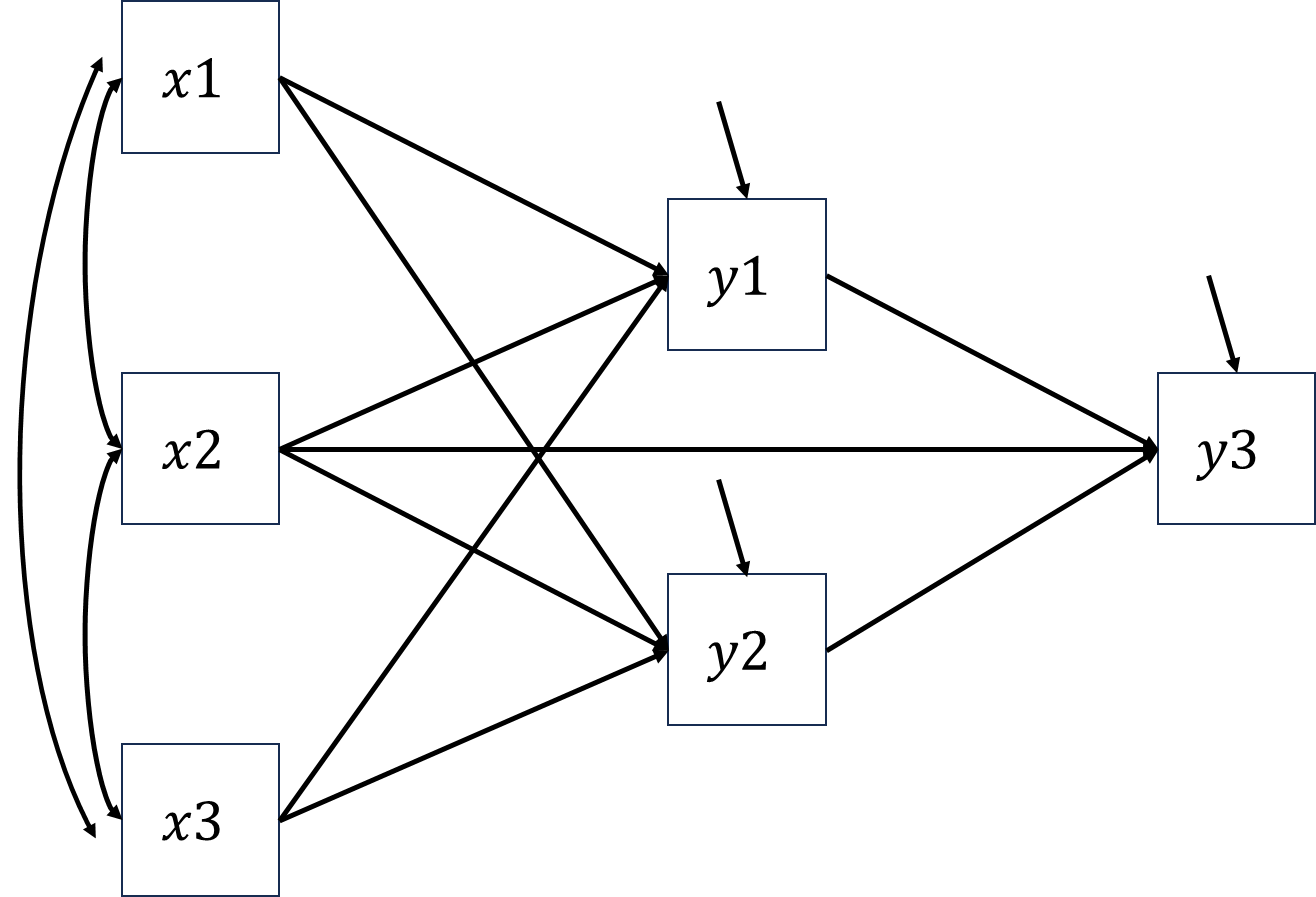
The corresponding element of $\mathbf{\Sigma }\mathbf{(}\mathit{\theta }\mathbf{)}$ are marked in red, $$\begin{array}{r}\left[\begin{array}{cccccc}{\sigma }_{x1}^2& & & & & \\ {\sigma }_{x2x1}& {\sigma }_{x2}^2& & & & \\ {\sigma }_{x3x1}& {\sigma }_{x3x1}& {\sigma }_{x3}^2& & & \\ {\sigma }_{y1x1}& {\sigma }_{y1x2}& {\sigma }_{y1x3}& {\sigma }_{y1}^2& & \\ {\sigma }_{y2x1}& {\sigma }_{y2x2}& {\sigma }_{y2x3}& {\sigma }_{y2y1}& {\sigma }_{y2}^2& \\ {\sigma }_{y3x1}& {\sigma }_{y3x2}& {\sigma }_{y3x3}& {\sigma }_{y3y1}& {\sigma }_{y3y2}& {\sigma }_{y3}^2\end{array}\right].\end{array}$$

Given the fact that there are $9$ slopes and $3$ residual variances to be estimated, $df=15-12=3$.

2.5 Homework

Derive the covariance structure of following model, assume $x$ is correlated with $w$

$$y={\beta }_{x}x+{\beta }_{w}w+{\beta }_{z}z+e$$