5  Moderation

As mentioned in the beginning of Chapter 4, moderation is another type of basic “causal” mechanisms we used to explain the relationship between $X$ and $Y$. But moderation is more complicated and less straight forward than mediation.

5.1 The simplest scenario: when moderator is continous

5.1.1 Basic moderation model

Consider a model where $X$ is assumed to affect/cause $Y$, the corresponding model is $$Y={\beta }_{1}X+ϵ.$$

Now we assume that the relationship between $X$ and $Y$ is moderated by a third variable $Z$, aka the moderator. A moderator is a qualitative (e.g., sex, race, class) or quantitative (e.g., level of reward) that affects the direction and/or strength of the relation between an independent or predictor variable and a dependent or criterion variable (Baron & Kenny, 1986, p. 1174).

The basic moderation model contains a product term $XZ$ representing the moderation effect $$Y={\beta }_0+{\beta }_{1}X+{\beta }_{2}Z+{\beta }_{3}XZ+ϵ$$

5.1.1.1 Non-zero mean structure

Note that, basic moderation model is a special case in which an intercept should always be included, i.e. the mean of $Y$ is not zero (Wen & Liu, 2020). $$\begin{array}{rl}\mathrm{cov}(X_1,X_2)& =E[(X_1-E(X_1))(X_2-E(X_2))]\\ & =E[X_1{X}_2-X_{1}E(X_2)-E(X_1)X_2+E(X_1)E(X_2)]\\ & =E(X_1{X}_2)-2E(X_1)E(X_2)+E(X_1)E(X_2)\\ E(X_1{X}_2)& =\mathrm{cov}(X_1,X_2)+E(X_1)E(X_2),\end{array}$$ therefore, it is easy to see that ${\beta }_0\ne 0$ even with all variables standardized $$\begin{array}{rl}E(Y)=0& ={\beta }_0+{\beta }_{1}E(X)+{\beta }_{2}E(Z)+{\beta }_{3}E(XZ)+E(ϵ)\\ 0& ={\beta }_0+0+0+{\beta }_3\mathrm{cov}(X,Z)+0\end{array}$$ this equation is solvable only if ${\beta }_0$ is non-zero. ${\beta }_0$ can be 0 only if $X$ and $Z$ are independent.

5.1.1.2 Centering

When doing moderation analysis, it is usually recommended to center the continuous independent variables (including all $X$s and $Z$) beforehand. There are two main reasons listed in past literature:

1. Centering variables makes interpretation easier.

For example, assume both $X$ and $Z$ are continuous, $CX$ and $CZ$ are the centered ones, the basic moderation model becomes

$$Y={\beta }_0+{\beta }_{1}CX+{\beta }_{2}CZ+{\beta }_{3}CX\times CZ+ϵ$$ where ${\beta }_1$ can be interpreted as the difference in the predicted value $\hat{Y}$ for each 1 unit change in $CX$, assuming $CZ=0$, which corresponds to the mean of $Z$. Thus ${\beta }_1$ is the simple main effect of $CX$ on $Y$ with $Z=\overline{Z}$.

2. Centering variables reduce non-essential multicollinearity. However, Olvera Astivia & Kroc (2019) has demonstrated that centering does not always reduce multicollinearity, making this argument less legislative.

Thus, centering is mainly for the interpretation purpose.

5.1.1.3 Why product term

Why does product term represent moderation effect?

$$\begin{array}{rl}Y& ={\beta }_0+{\beta }_{1}X+{\beta }_{2}Z+{\beta }_{3}XZ+ϵ\\ & ={\beta }_0+({\beta }_1+{\beta }_{3}Z)X+{\beta }_{2}Z+ϵ,\end{array}$$ it is easy to see that, by adding a product term, $Z$ becomes part of the slope of $X$, thus the value of $Z$ impacts the relationship between $X$ and $Y$. For example, if $Z$ is a dichotomous variable such as gender with value equals to either $0$ (male) and $1$ (female), we shall have $$\begin{array}{r}\{\begin{array}{l}y={\beta }_0+{\beta }_{1}X+ϵ,Z=0\\ y={\beta }_0+({\beta }_1+{\beta }_3)X+{\beta }_2+ϵ,Z=1\end{array}\end{array}$$

$Z$ is said to alter the strength of the relationship between $X$ and $Y$, As long as ${\beta }_3$ is significantly different from 0.

5.1.1.4 Moderation effect vs Interaction effect

What is the difference between the interaction effect and moderation effect?

Normally, these two effects are equivalent.

In the context of two-way ANOVA, interaction effect is the effect of two IVs (factors A and B) on one DV (Y). Interaction effect exists when the pattern of the relationship of one IV on DV depends on the level of another IV. As long as $F_{AB}$ is statistically significant, we observed strong evidence that support the interaction effect.

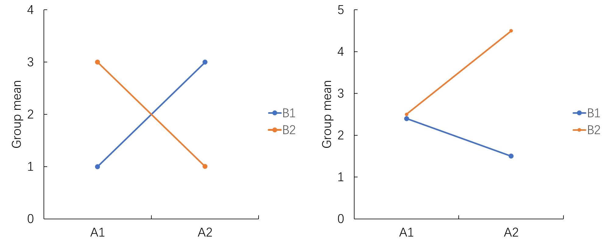
The interaction effect can be illustrated by testing the two simple effects of either A or B. For example, in the right panel of the figure above, the simple effect of B is insignificant at A1, whereas the simple effect of B is significant at A2, the pattern of the relationship between B and Y depends on A. Or equivalently, the simple effect of A is significant (A1>A2) at B1, whereas the simple effect of A is also significant (A1<A2) at B2, the pattern of the relationship between A and Y depends on B.

But in practice, the choice regarding which pair of simple effects to report is purely theory-driven. For example, in the figure above, we cares more about the simple effect of B, that is, A alters the strength of the relationship between B and Y. In this case, A is effectively a moderator, interaction effect of A and B on Y is equivalent to the moderation effect of A on the relationship of B on Y.

In the context of basic moderation, as long as ${\beta }_3$ is statistically significant, we observe strong evidence that favors the existence of moderation effect. However, the moderation effect can be illustrated by either treating $X$ as the moderator, or $Z$ as the moderator. Because $$\begin{array}{rl}Y& ={\beta }_0+{\beta }_{1}X+{\beta }_{2}Z+{\beta }_{3}XZ+ϵ\\ & ={\beta }_0+({\beta }_1+{\beta }_{3}Z)X+{\beta }_{2}Z+ϵ\\ & ={\beta }_0+({\beta }_2+{\beta }_{3}X)Z+{\beta }_{1}X+ϵ.\end{array}$$ Therefore, just like interpreting interaction effect, in practice, the determination of moderator is purely theory-driven.

5.1.1.5 Two types of path diagram

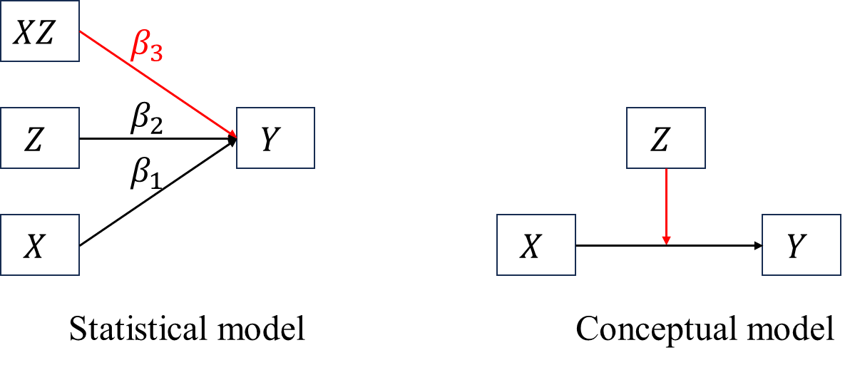
There exist two path diagrams for a basic moderation model (see the figure below), the left one represents the statistical model, corresponding to $$\begin{array}{rl}Y& ={\beta }_0+{\beta }_{1}X+{\beta }_{2}Z+{\beta }_{3}XZ+ϵ,\end{array}$$ of which the moderator can be either $X$ or $Z$; the right one represents the theory-driven conceptual model, wherein the moderator is clearly defined as $Z$ according to theory. Statistical model always underlies conceptual model. Conceptual model is more frequently used in empirical research, whereas statistical model is the key when writting analysis syntax.

5.1.2 Moderation analysis: simple slope analysis and visualization

5.1.2.1 Continuous $X$

In moderation analysis, we interest the most in the moderation effect, i.e. ${\beta }_3$. Therefore the null hypothesis in moderation analysis is

$$H_0:{\beta }_3=0$$

In factorial two-way ANOVA, an significant interaction effect only implies that the population means of all cells are very likely different, but the specific pattern remains unknown. We need to conduct simple effect analysis and visualize the interaction effect.

Similarly, in moderation analysis, the significance of $\widehat{{\beta }_3}$ fails to provide information about the pattern of moderation effect. We need to conduct the simple slope analysis and visualize the moderation effect.

The essence of moderation effect is that the slope of $X$ on $Y$ depends on $Z$. Simple slope is just simple main effect, the slope of $X$ on $Y$ at a certain level of $Z$.

The simple slope of a basic moderation model is ${\beta }_1+{\beta }_{3}Z$, the common NHST is the $t$-test

$$t=\frac{\widehat{{\beta }_1}+\widehat{{\beta }_3}Z}{\sqrt{\text{var}(\widehat{{\beta }_1})+2Z\text{cov}(\widehat{{\beta }_1},\widehat{{\beta }_3})+Z^2\text{var}(\widehat{{\beta }_3})}}$$ with $$H_0:{\beta }_1+{\beta }_{3}Z=0,$$ and $df=N-K-1$, where $K$ is the number of independent variables (including the product term).

It is clear that the number of simple slopes vary according to the nature of moderator. With categorical moderator, we shall have fixed number of simple slopes; with continuous moderator, we shall have infinite number of simple slopes. For continuous moderator, a popular method is pick-a-point (Rogosa, 1980). The most frequently used 3 points are $Z_1=\overline{Z}$, $Z_2=\overline{Z}+S{D}_Z$, and $Z_3=\overline{Z}-S{D}_Z$, therefore we need to perform 3 $t$-tests.

#> [1] 1.429384

ABCDEFGHIJ0123456789

	lhs <chr>	op <chr>	rhs <chr>	label <chr>	est <dbl>	se <dbl>	z <dbl>	pvalue <dbl>	ci.lower <dbl>
15	SSHigh	:=	b1+b3*1.429	SSHigh	1.4374781	0.1691846	8.496507	0.000000e+00	1.1058824
16	SSMod	:=	b1+b3*0	SSMod	0.5548651	0.1053937	5.264692	1.404247e-07	0.3482973
17	SSLow	:=	b1+b3*(-1.429)	SSLow	-0.3277478	0.1263960	-2.593023	9.513644e-03	-0.5754795

3 rows | 1-10 of 11 columns

• Johoson-Neyman test

Johnson & Neyman (1936) proposed another test for continuous moderator. Because $Z$ is continuous, we have infinite simple slopes to test, each one correspond to a $t$ upon which we calculate the $p$-value. Thus, we would like to know the range of $Z$, in which all possible $Z$s have significant $t$s.

From the aforementioned $t$-test formula, we have $$\begin{array}{rl}\left|\frac{\widehat{{\beta }_1}+\widehat{{\beta }_3}Z}{\sqrt{\text{var}(\widehat{{\beta }_1})+2Z\text{cov}(\widehat{{\beta }_1},\widehat{{\beta }_3})+Z^2\text{var}(\widehat{{\beta }_3})}}\right|& >t_c\\ t_c^2\text{var}(\widehat{{\beta }_1})+2t_c^{2}Z\text{cov}(\widehat{{\beta }_1},\widehat{{\beta }_3})+t_c^2{Z}^2\text{var}(\widehat{{\beta }_3})& <\widehat{{\beta }_1^2}+2\widehat{{\beta }_1}\widehat{{\beta }_3}Z+\widehat{{\beta }_3^2}{Z}^2\end{array}$$ where $t_c$ is the right-tail critical value of $t$ distribution with given $df$. It is easy to see that the last equation above is effectively a second order inequality of $Z$ and can be rewritten as

$$[t_c^2\text{var}(\widehat{{\beta }_3})-\widehat{{\beta }_3^2}]Z^2+[2t_c^2\text{cov}(\widehat{{\beta }_1},\widehat{{\beta }_3})-2\widehat{{\beta }_1}\widehat{{\beta }_3}]Z+[t_c^2\text{var}(\widehat{{\beta }_1})-\widehat{{\beta }_1^2}]<0.$$

Let’s denote $t_c^2\text{var}(\widehat{{\beta }_3})-\widehat{{\beta }_3^2}=a$, $2t_c^2\text{cov}(\widehat{{\beta }_1},\widehat{{\beta }_3})-2\widehat{{\beta }_1}\widehat{{\beta }_3}=b$, and $t_c^2\text{var}(\widehat{{\beta }_1})-\widehat{{\beta }_1^2}=c$, the roots of $a{Z}^2+bZ+c<0$ are $$Z=\frac{-b\pm \sqrt{b^2-4ac}}{2a}.$$ The $Z$s with significant simple slope are all in the intersection area (shaded) that between the graph of $f(Z)=a{Z}^2+bZ+c$ and $y<0$. It could be one area when $a>0$ or two areas when $a<0$.

For linear regression with fixed $x$, one can use the following code

library(interactions)

#> Warning: package 'interactions' was built under R version 4.3.3

res_lm <- lm(data = df_cont, formula = "Y~X*Z")
johnson_neyman(res_lm, pred = "X", modx = "Z", alpha = 0.05)

#> JOHNSON-NEYMAN INTERVAL
#> 
#> When Z is OUTSIDE the interval [-1.29, -0.56], the slope of X is p < .05.
#> 
#> Note: The range of observed values of Z is [-2.85, 3.10]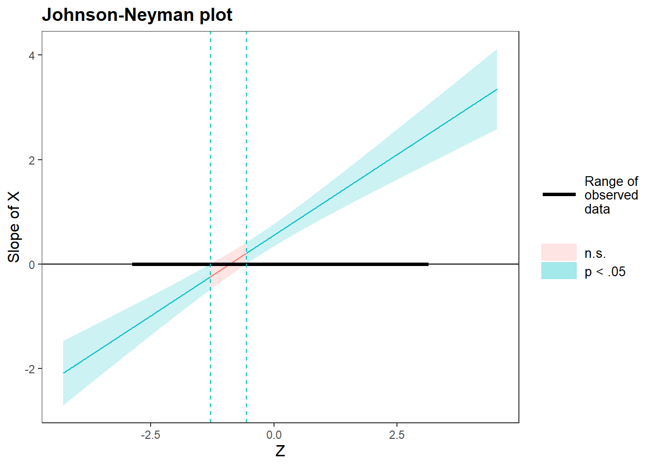

For SEM-based approach, one can extract $t_c$ and all required parameters estimate from the output of lavaan and manually calculate $a$, $Z_1$ and $Z_2$.

5.1.2.2 Categorical $X$

Suppose $X$ is a 3-level categorical variable and is dummy coded, the 1st category is used as the reference. The basic moderation model becomes $$\begin{array}{rl}Y& ={\beta }_0+{\beta }_1{d}_{2}X+{\beta }_2{d}_{3}X+{\beta }_{3}Z+{\beta }_4{d}_{2}XZ+{\beta }_5{d}_{3}XZ+ϵ\\ & ={\beta }_0+{\beta }_{3}Z+({\beta }_1+{\beta }_{4}Z)d_{2}X+({\beta }_2+{\beta }_{5}Z)d_{3}X+ϵ.\end{array}$$ When $X=1$, $d_{2}X=0=d_{3}X=0$, we have $$\begin{array}{rl}Y& ={\beta }_0+{\beta }_{3}Z+ϵ.\end{array}$$ When $X=2$, $d_{2}X=1$, $d_{3}X=0$, we have $$\begin{array}{rl}Y& ={\beta }_0+{\beta }_1+({\beta }_3+{\beta }_4)Z+ϵ.\end{array}$$ When $X=3$, $d_{2}X=0$, $d_{3}X=1$, we have $$\begin{array}{rl}Y& ={\beta }_0+{\beta }_2+({\beta }_3+{\beta }_5)Z+ϵ.\end{array}$$ Assume that all coefficients are significant. It is easy to see that if we removed the terms containing $Z$, the predicted value of $Y$ depends on $X$, implying that $X$ has an effect on $Y$. After introducing $Z$, the predicted value of $Y$ given $X$ becomes a function of $Z$, i.e. the effect of $X$ on $Y$ is moderated by $Z$.

5.2 When moderator is categorical

5.2.1 Continuous $X$

When moderator is a 3-level categorical variable with the 1st category as reference we have $$\begin{array}{rl}Y& ={\beta }_0+{\beta }_{1}X+{\beta }_2{d}_{2}Z+{\beta }_3{d}_{3}Z+{\beta }_{4}X{d}_{2}Z+{\beta }_{5}X{d}_{3}Z+ϵ,\end{array}$$ in the moderation above, there are 3 simple slopes to be tested,

• for $Z=1$, we have $Y={\beta }_0+{\beta }_{1}X$,
• for $Z=2$, we have $Y={\beta }_0+{\beta }_2+({\beta }_1+{\beta }_4)X$.
• for $Z=3$, we have $Y={\beta }_0+{\beta }_3+({\beta }_1+{\beta }_5)X$.

For example,

ABCDEFGHIJ0123456789

	X <dbl>	d_Z_1 <dbl>	d_Z_2 <dbl>	d_Z_3 <dbl>	Xd_Z_1 <dbl>	Xd_Z_2 <dbl>	Xd_Z_3 <dbl>	Y <dbl>
1	-0.56047565	1	0	0	-0.56047565	0	0	-0.4954800
2	-0.23017749	1	0	0	-0.23017749	0	0	-0.3677777
3	1.55870831	1	0	0	1.55870831	0	0	0.3408155
4	0.07050839	1	0	0	0.07050839	0	0	-0.5172591
5	0.12928774	1	0	0	0.12928774	0	0	0.1274843
6	1.71506499	1	0	0	1.71506499	0	0	1.6887117

6 rows

ABCDEFGHIJ0123456789

	lhs <chr>	op <chr>	rhs <chr>	label <chr>	est <dbl>	se <dbl>	z <dbl>	pvalue <dbl>	ci.lower <dbl>
1	Y	~	X	b1	0.4498383	0.1080804	4.162069	3.153765e-05	0.2380045
2	Y	~	d_Z_2	b2	0.6231661	0.1395988	4.463979	8.045144e-06	0.3495575
3	Y	~	d_Z_3	b3	0.4872201	0.1397282	3.486913	4.886307e-04	0.2133578
4	Y	~	Xd_Z_2	b4	0.4165192	0.1486292	2.802406	5.072307e-03	0.1252114
5	Y	~	Xd_Z_3	b5	0.5681581	0.1498965	3.790336	1.504437e-04	0.2743663

5 rows | 1-10 of 11 columns

The whole moderation model is $$\hat{Y}=0.468+0.450X+0.623dZ2+0.487dZ3+0.417XdZ2+0.568XdZ3,$$ thus,

• for $Z=1$, we have $\hat{Y}=0.468+0.450X$,
• for $Z=2$, we have $\hat{Y}=0.468+0.623+(0.450+0.417)X$.
• for $Z=3$, we have $\hat{Y}=0.468+0.487+(0.450+0.568)X$.

k <- 5
pars <- parameterestimates(res)
# simple slope when Z = 1
b1 <- pars$est[[1]]
b4 <- pars$est[[4]]
b5 <- pars$est[[5]]
var_b1 <- pars$se[[1]]^2
var_b4 <- pars$se[[4]]^2
var_b5 <- pars$se[[5]]^2
cov_b1b4 <- vcov(res)["b1", "b4"]
cov_b1b5 <- vcov(res)["b1", "b5"]
t_Z1 <- b1/sqrt(var_b1)
p_Z1 <- 2*min(
  pt(t_Z1, df = n - k - 1), 
  pt(t_Z1, df = n - k - 1, lower.tail = FALSE)
)
# simple slope when Z = 2
t_Z2 <- (b1 + b4)/sqrt(var_b1 + 2*cov_b1b4 + var_b4)
p_Z2 <- 2*min(
  pt(t_Z2, df = n - k - 1), 
  pt(t_Z2, df = n - k - 1, lower.tail = FALSE)
)
# simple slope when Z = 3
t_Z3 <- (b1 + b5)/sqrt(var_b1 + 2*cov_b1b5 + var_b5)
p_Z3 <- 2*min(
  pt(t_Z3, df = n - k - 1), 
  pt(t_Z3, df = n - k - 1, lower.tail = FALSE)
)
test_simple_slope <- data.frame(
  t = c(t_Z1, t_Z2, t_Z3),
  p = c(p_Z1, p_Z2, p_Z3)
)
print(test_simple_slope)
#>          t            p
#> 1 4.162069 4.146295e-05
#> 2 8.491557 1.026076e-15
#> 3 9.801312 8.262378e-20

To avoid calculate $t$ manually for the rest 2 simple slopes, we can just switch the reference group.

# category 2 as reference
model_Z2 <- "
  Y ~ b1*X + b2*d_Z_1 + b3*d_Z_3 + b4*Xd_Z_1 + b5*Xd_Z_3
"
res_model_Z2 <- sem(
  model = model_Z2, 
  data = df_cate,
  meanstructure = TRUE
)
parameterestimates(res_model_Z2)[1:5, ]

ABCDEFGHIJ0123456789

	lhs <chr>	op <chr>	rhs <chr>	label <chr>	est <dbl>	se <dbl>	z <dbl>	pvalue <dbl>	ci.lower <dbl>
1	Y	~	X	b1	0.8663575	0.1020258	8.4915571	0.000000e+00	0.6663907
2	Y	~	d_Z_1	b2	-0.6231661	0.1395988	-4.4639790	8.045144e-06	-0.8967747
3	Y	~	d_Z_3	b3	-0.1359460	0.1398174	-0.9723112	3.308958e-01	-0.4099830
4	Y	~	Xd_Z_1	b4	-0.4165192	0.1486292	-2.8024055	5.072307e-03	-0.7078271
5	Y	~	Xd_Z_3	b5	0.1516388	0.1455913	1.0415374	2.976262e-01	-0.1337149

5 rows | 1-10 of 11 columns

# category 3 as reference
model_Z3 <- "
  Y ~ b1*X + b2*d_Z_1 + b3*d_Z_2 + b4*Xd_Z_1 + b5*Xd_Z_2
"
res_model_Z3 <- sem(
  model = model_Z3, 
  data = df_cate,
  meanstructure = TRUE
)
parameterestimates(res_model_Z3)[1:5, ]

ABCDEFGHIJ0123456789

	lhs <chr>	op <chr>	rhs <chr>	label <chr>	est <dbl>	se <dbl>	z <dbl>	pvalue <dbl>	ci.lower <dbl>
1	Y	~	X	b1	1.0179963	0.1038633	9.8013120	0.0000000000	0.8144280
2	Y	~	d_Z_1	b2	-0.4872201	0.1397282	-3.4869128	0.0004886307	-0.7610824
3	Y	~	d_Z_2	b3	0.1359460	0.1398174	0.9723112	0.3308957772	-0.1380910
4	Y	~	Xd_Z_1	b4	-0.5681581	0.1498965	-3.7903359	0.0001504437	-0.8619498
5	Y	~	Xd_Z_2	b5	-0.1516388	0.1455913	-1.0415374	0.2976261849	-0.4369926

5 rows | 1-10 of 11 columns

Manually visualize the moderation effect.

x <- range(df_cate$X)
x <- rep(x, times = 3)
y <- rep(0, times = 6)
y[1:2] <- 0.468 + x[1:2]*0.450
y[3:4] <- 0.468 + 0.628 + (0.450 + 0.417)*x[3:4]
y[5:6] <- 0.468 + 0.487 + (0.450 + 0.568)*x[5:6]
df_plot <- data.frame(
  x, y, z = rep(1:3, each = 2)
)
df_plot$z <- factor(df_plot$z)
ggplot(df_plot, aes(x = x, y = y, color = z)) + 
  geom_line()

If using linear regression with fixed $x$ to fit a basic moderation model, the interactions package could be used to visualize interaction effect.

5.2.2 Categorical $X$

When $X$ and $Z$ are categorical, we just use ANOVA to conduct moderation analysis.

5.3 Typical procedures of moderation analysis

In summary, the typical procedures of moderation analysis are:

1. center or standardize continuous independent variables, if any;
2. dummy code categorical variables, if any;
3. construct product term;
4. test significance of ${\beta }_3$;
5. simple slope analysis and visualization.

5.4 Real data example

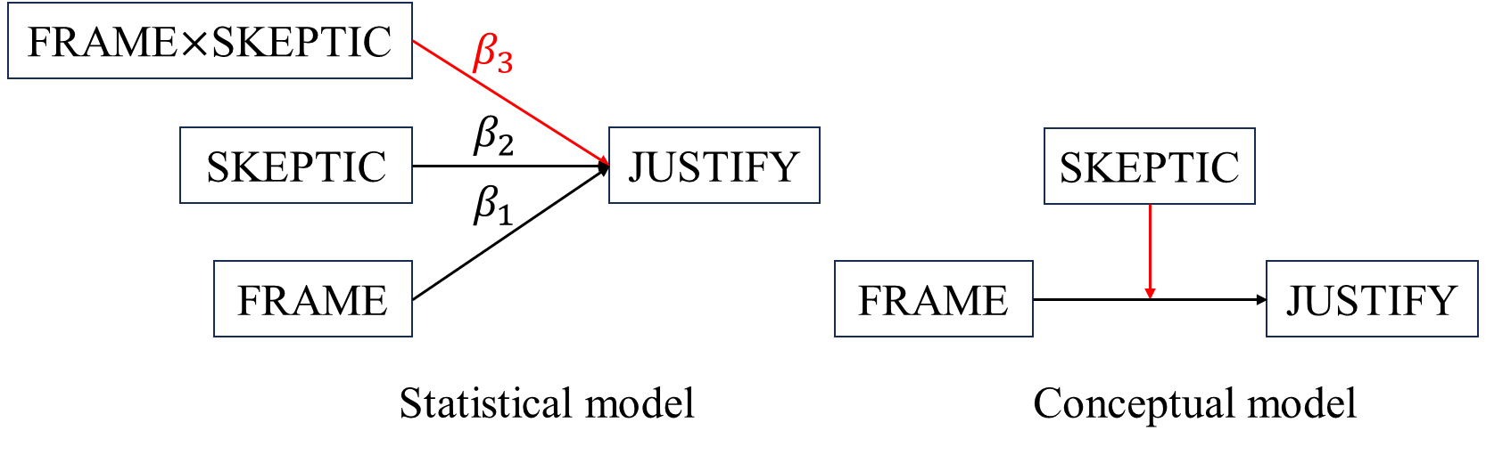
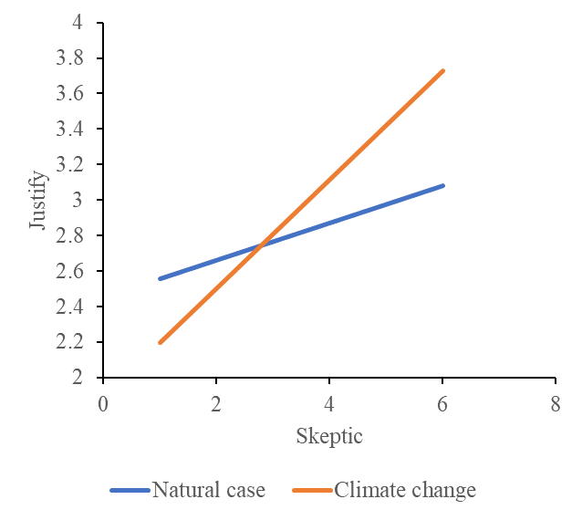
The following example is from Hayes (2017) (p245). In this study (Chapman & Lickel, 2016), 211 participants read a news story about a famine in Africa that was reportedly caused by severe droughts affecting the region. For half of the participants, the story attributed the droughts to the effects of climate change, whereas for the other half, the story provided no information suggesting that climate change was responsible for the droughts. I refer to these as the “climate change” and “natural causes” conditions, respectively. They are coded in a variable named FRAME in the data, which is set to 0 for those in the natural causes condition and 1 for those in the climate change condition.

After reading this story, the participants were asked a set of questions assessing how much they agreed or disagreed with various justifications for not providing aid to the victims, for example, that they did not deserve help, that the victims had themselves to blame for their situation, that the donations would not be helpful or effective, and so forth. Responses to these questions were aggregated and are held in a variable named JUSTIFY that quantifies the strength of a participant’s justifications for withholding aid. So higher scores on JUSTIFY reflect a stronger sense that helping out the victims was not justified. The participants also responded to a set of questions about their beliefs about whether climate change is a real phenomenon. This measure of climate change skepticism is named SKEPTIC in the data, and the higher a participant’s score, the more skeptical he or she is about the reality of climate change.

The purpose of this analysis is to examine whether framing the disaster as caused by climate change rather than leaving the cause unspecified influences people’s justifications for not helping, and also whether this effect of framing is dependent on a person’s skepticism about climate change.

• $X$ independent variable: FRAME, categorical, 0 natural case condition, 1 climate change condition
• $Y$ dependent variable: JUSTIFY, continuous
• $Z$ moderator: SKEPTIC, continuous

$$\hat{Y}=2.452-0.562X+0.105Z+0.201XZ$$ For participants in the natural case condition ($X=0$), $$\begin{array}{r}\{\begin{array}{ll}\hat{Y}=2.452+0.105\times 2=2.662& \text{if }Z=2\\ \hat{Y}=2.452+0.105\times 3.5=2.8195& \text{if }Z=3.5\\ \hat{Y}=2.452+0.105\times 5=2.977& \text{if }Z=5,\end{array}\end{array}$$ for participants in the climate change condition ($x=1$), $$\begin{array}{r}\{\begin{array}{ll}\hat{Y}=2.452-0.562+0.105\times 2+0.201\times 2=2.502& \text{if }Z=2\\ \hat{Y}=2.452-0.562+0.105\times 3.5+0.201\times 3.5=2.961& \text{if }Z=3.5\\ \hat{Y}=2.452-0.562+0.105\times 5+0.201\times 5=3.420& \text{if }Z=5,\end{array}\end{array}$$ From these calculations, it appears that participants lower in climate change skepticism reported weaker justifications for withholding aid when told the drought was caused by climate change compared to when not so told. However, among those at the higher end of the continuum of climate change skepticism, the opposite is observed. Participants high in skepticism about climate change who read the story attributing the drought to climate change reported stronger justifications for withholding aid than those who read the story that did not attribute the drought to climate change.

5.5 How to report moderation analysis

• Continuous Z:
  • Section 2.1.3 in Zhao et al. 2024
  • Johoson-Neyman: section 3.4 in Hu et al. 2023
  • Section 3.3
• Categorical Z and categorical X: Section 3.1
• Categotical Z and continuous X: Section 3.2

Chapman, D. A., & Lickel, B. (2016). Climate change and disasters: How framing affects justifications for giving or withholding aid to disaster victims. Social Psychological and Personality Science, 7(1), 13–20.

Hayes, A. F. (2017). Introduction to mediation, moderation, and conditional process analysis: A regression-based approach. Guilford publications.

Johnson, P. O., & Neyman, J. (1936). Tests of certain linear hypotheses and their application to some educational problems. Statistical Research Memoirs.

Olvera Astivia, O. L., & Kroc, E. (2019). Centering in multiple regression does not always reduce multicollinearity: How to tell when your estimates will not benefit from centering. Educational and Psychological Measurement, 79(5), 813–826.

Rogosa, D. (1980). A critique of cross-lagged correlation. Psychological Bulletin, 88(2), 245.

Wen, Z., & Liu, H. (2020). Mediation effect and moderation effect: Method and application. Educational Science Publishing House.