4  Mediation

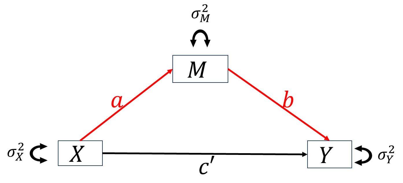
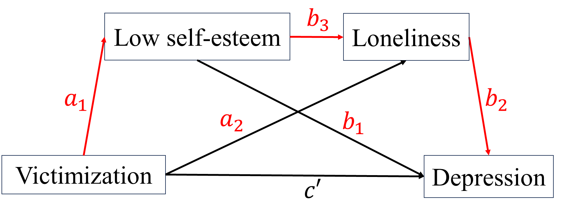
When studying the relationship between independent variable $X$ and dependent variable $Y$, we want to know how $X$ impact $Y$. For this purpose, researchers proposed two types of basic “causal” mechanisms between $X$ and $Y$, mediation and moderation.

4.1 The simplest scenario: when everything is continuous

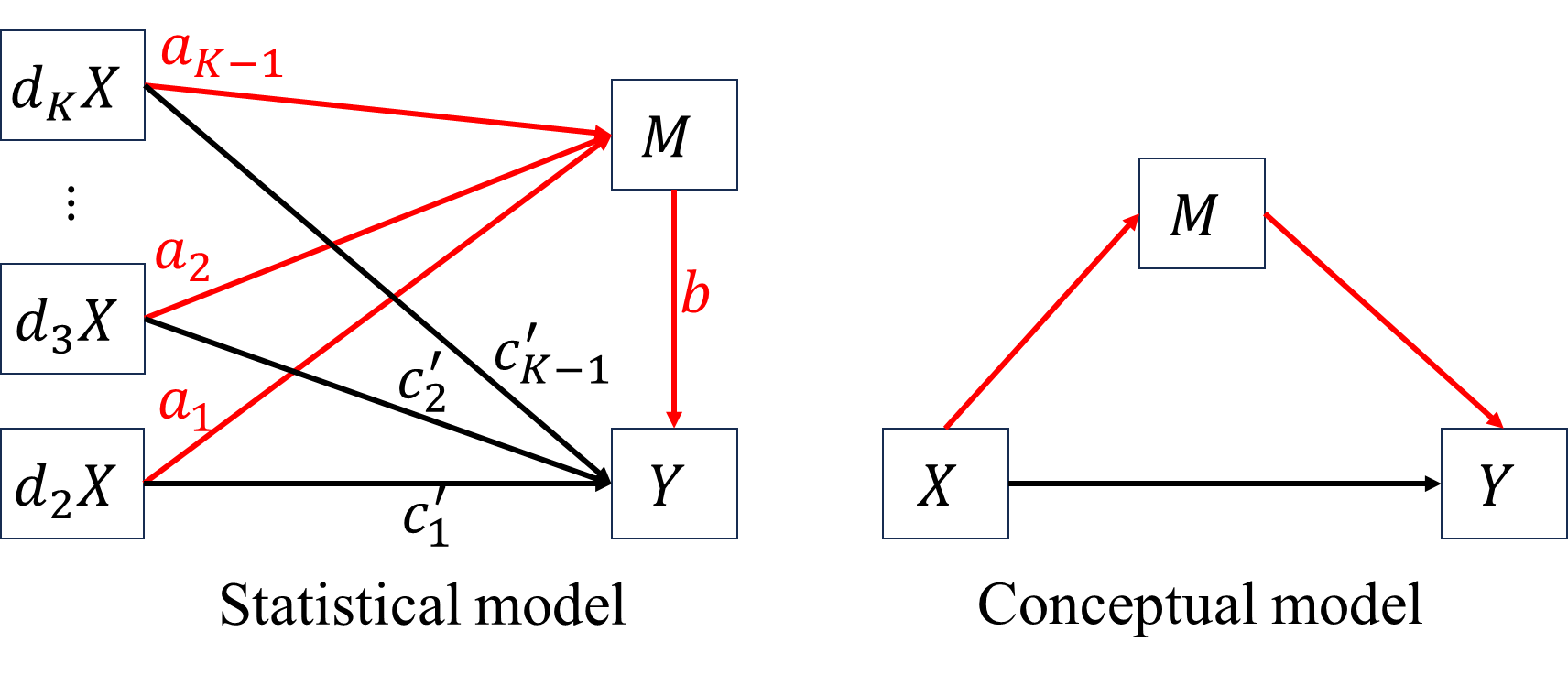
4.1.1 Basic mediation model

Consider a model where $X$ is assumed to affect/cause $Y$, $x$ and $y$ are both continuous.

the corresponding model is $Y=cX+{ϵ}_Y.$

More specifically, we assume $X$ affects $Y$ through a third continuous variable $M$, following is the resulting statistical model and conceptual model

the corresponding equations are $$\begin{array}{rl}M& =aX+{ϵ}_M\\ Y& =bM+c^{\prime }X+{ϵ}_Y,\end{array}$$ where $c^{\prime }$ is called the direct effect of $X$ on $Y$. The effect of $X$ on $Y$ through $M$ is called the mediation effect or indirect effect, which is $ab$. The total effect of $X$ on $Y$ is $c=ab+c^{\prime }$, but why?

It is easy to see that $$Y=(ab+c^{\prime })X+b{ϵ}_M+{ϵ}_Y,$$

meaning that the effect of $X$ on $Y$ after including the mediator $M$ is now $ab+c^{\prime }$. The resulting $\mathbf{\Sigma }(\mathit{\theta })$ is $$\begin{array}{r}\left[\begin{array}{ccc}{\sigma }_X^2& {\sigma }_{XM}& {\sigma }_{XY}\\ {\sigma }_{MX}& {\sigma }_M^2& {\sigma }_{MY}\\ {\sigma }_{YX}& {\sigma }_{MY}& {\sigma }_Y^2\end{array}\right],\end{array}$$ where $$\begin{array}{rl}{\sigma }_{XM}& =a{\sigma }_X^2\\ {\sigma }_M^2& =a^2{\sigma }_X^2+{\sigma }_{{ϵ}_M}^2\\ {\sigma }_{XY}& =b{\sigma }_{XM}+c^{\prime }{\sigma }_X^2\\ & =(ab+c^{\prime }){\sigma }_X^2\\ {\sigma }_{MY}& =b{\sigma }_M^2+c^{\prime }{\sigma }_{XM}\\ & =b{\sigma }_M^2+a{c}^{\prime }{\sigma }_X^2\\ & =(ab+c^{\prime })a{\sigma }_X^2+b{\sigma }_{{ϵ}_M}^2\\ {\sigma }_Y^2& =b^2{\sigma }_M^2+c^{\prime 2}{\sigma }_X^2+{\sigma }_{{ϵ}_Y}^2+2b{c}^{\prime }{\sigma }_{XM}\\ & =a^2{b}^2{\sigma }_X^2+b{\sigma }_{{ϵ}_M}^2+c^{\prime 2}{\sigma }_X^2+2ab{c}^{\prime }{\sigma }_X^2+{\sigma }_{{ϵ}_Y}^2\\ & =(ab+c^{\prime }{)}^2{\sigma }_X^2+b^2{\sigma }_{{ϵ}_M}^2+{\sigma }_{{ϵ}_Y}^2\end{array}$$

• Complete mediation: $c^{\prime }=0$
• Partial mediation: $c^{\prime }\ne 0$

Important remarks:

• Basic mediation model is a saturated model, it is statistically equivalent to any saturated model (e.g. regression model $Y={\beta }_0+{\beta }_{1}X+{\beta }_{2}M+{ϵ}_y$, or switch $X$ and $M$), therefore it is a theoretically defined model,
• If the presumed mediation model is not theoretically correct, the results from mediation analysis are nonsense.

4.1.2 Mediation analysis

In mediation model, we interest the most in mediating effect, i.e. $ab$. Therefore the null hypothesis in mediation analysis is

$$ab=0$$ or

$$c-c^{\prime }=0$$

It is recommended to perform a single null hypothesis significance testing (NHST) of $ab$. Several methods available.

4.1.2.1 Sobel test

Sobel (1982) proposed to test the significance of $ab$ via a $Z$ test, where$Z=\frac{\widehat{ab}-0}{s{e}_{\widehat{ab}}}$, $s{e}_{\hat{a}\hat{b}}=\sqrt{{\hat{b}}^2{s}_a^2+{\hat{a}}^2{s}_b^2}$. The Sobel test is easy to conduct, however,

• The derivation of the Sobel $s{e}_{\hat{a}\hat{b}}$ assumes that $a$ and $b$ are independent, which may not be true
• The Sobel test assumes $ab$ is normally distributed, which may not be true, especially when $n$ is small.

Thus Sobel test has been shown very conservative with low power. One of the most popular alternative of the Sobel test is the bootstrap method.

4.1.2.2 Bootstrap methods

StatsQuest’s bootstrap main idea video

4.1.2.2.1 Ordinary bootstrap, aka non-parametric bootstrap

The sampling distribution of test statistic is a must-have for NHST. Usually, we could have a theoretically distribution with precise numerical probability density function. However, this is not always the case. The distribution of a statistic can be too complex to have a clearly defined function form. What’s more, in real data analysis, even if the theoretical distribution of test statistic is available, we may not have large enough sample size for stable inference. Therefore, we use bootstrap to directly generate an empirical distribution. The basic procedures of bootstraping are as following:

1. Treat the original data (sample size = $n$) set as population. Draw a bootstrap sample of $n$ observations randomly with replacement from the population,
2. Use the bootstrap sample, estimate the parameters $\theta$ in interest,
3. Repeat steps 1 and 2 for a total of $B$ times, $B$ is the number of bootstrap samples,
4. Construct the standard error and confident interval of $\theta$.

In the case of testing $ab$, the standard error of $\widehat{ab}$ can be calculated as

$$s{e}_{\hat{a}\hat{b}}=\sqrt{\frac{\sum _{bt=1}^B({\hat{a}}^{bt}{\hat{b}}^{bt}-mean(\hat{a}\hat{b}))}{B-1}},$$ where

$$mean(\hat{a}\hat{b})=\frac{\sum _{bt=1}^B{\hat{a}}^{bt}{\hat{b}}^{bt}}{B}$$ The $1-\alpha$ percentile interval is

$$[({\hat{a}}^{bt}{\hat{b}}^{bt}{)}_{P_{\alpha /2}},({\hat{a}}^{bt}{\hat{b}}^{bt}{)}_{P_{1-\alpha /2}}].$$

4.1.2.2.2 Parametric bootstrap

The only difference between non-parametric bootstrapping and parametric bootstrapping is the way how bootstrapping sample is generated.

In non-parametric bootstrapping, we treat the raw data as population and resample directly from this population with replacement to construct bootstrap sample.

In parametric bootstrapping, we use a model-based approach. More specifically, we now assume that the model we test is the underlying data generation model for the raw data. Based on this model, usually containing distributional assumption, we can derive a estimated population and generate pseudo-data as bootstrap sample directly from this population.

Let’s draw a sample from a $N(60,8)$ normal distribution

set.seed(123)
x <- rnorm(18, mean = 60, sd = 8)
x

#>  [1] 55.51619 58.15858 72.46967 60.56407 61.03430 73.72052 63.68733 49.87951
#>  [9] 54.50518 56.43470 69.79265 62.87851 63.20617 60.88546 55.55327 74.29531
#> [17] 63.98280 44.26706

mean(x)

#> [1] 61.15729

sd(x)

#> [1] 8.066665

In non-parametric bootstrapping,

n <- length(x)
n_bootstrap <- 100
x_bootstrap <- matrix(0, nrow = n_bootstrap, ncol = n)
for (i in 1:n_bootstrap) {
  x_bootstrap[i, ] <- sample(x, n, replace = TRUE)
}
head(x_bootstrap)

#>          [,1]     [,2]     [,3]     [,4]     [,5]     [,6]     [,7]     [,8]
#> [1,] 69.79265 63.68733 62.87851 55.55327 56.43470 63.20617 63.68733 54.50518
#> [2,] 55.51619 73.72052 55.55327 54.50518 55.55327 74.29531 73.72052 69.79265
#> [3,] 60.88546 72.46967 49.87951 74.29531 62.87851 60.88546 72.46967 60.88546
#> [4,] 56.43470 62.87851 60.88546 63.98280 60.88546 72.46967 49.87951 60.88546
#> [5,] 73.72052 74.29531 69.79265 60.56407 62.87851 60.88546 63.68733 54.50518
#> [6,] 69.79265 74.29531 49.87951 72.46967 60.56407 62.87851 63.98280 56.43470
#>          [,9]    [,10]    [,11]    [,12]    [,13]    [,14]    [,15]    [,16]
#> [1,] 54.50518 56.43470 63.68733 73.72052 58.15858 61.03430 49.87951 62.87851
#> [2,] 49.87951 63.68733 74.29531 63.98280 44.26706 63.98280 58.15858 60.56407
#> [3,] 63.68733 72.46967 55.55327 61.03430 49.87951 56.43470 44.26706 56.43470
#> [4,] 55.55327 63.98280 69.79265 63.68733 55.55327 73.72052 60.88546 63.68733
#> [5,] 63.68733 58.15858 74.29531 63.20617 55.55327 63.68733 60.56407 55.51619
#> [6,] 69.79265 49.87951 60.88546 63.20617 58.15858 69.79265 63.20617 60.88546
#>         [,17]    [,18]
#> [1,] 63.20617 44.26706
#> [2,] 63.20617 61.03430
#> [3,] 62.87851 58.15858
#> [4,] 56.43470 61.03430
#> [5,] 49.87951 74.29531
#> [6,] 73.72052 49.87951

In reality, we will know nothing about the underlying distribution, let alone $\mu =60$, $sd=8$. But we can make assumption. By assuming that our sample is normally distributed, we are actually fit our data with a statistical model with normal distribution assumption and only two parameters $\mu$ and $sd$. Now we have $\hat{\mu }$ and $\widehat{sd}$, we can have a estimated population $N(\hat{\mu },\widehat{sd})$ and directly sampling from it.

par_mean <- mean(x)
par_sd <- sd(x)
x_bootstrap_para <- matrix(0, nrow = n_bootstrap, ncol = n)
for (i in 1:n_bootstrap) {
  x_bootstrap_para[i, ] <- rnorm(n, mean = par_mean, sd = par_sd)
}
head(x_bootstrap_para)

#>          [,1]     [,2]     [,3]     [,4]     [,5]     [,6]     [,7]     [,8]
#> [1,] 74.67357 68.53801 70.38768 68.44050 64.99213 56.45823 56.85829 48.24385
#> [2,] 64.77606 74.68124 58.64473 68.04313 44.25913 57.06544 50.73509 70.13842
#> [3,] 70.10338 56.55200 45.98042 51.67333 68.84125 58.81338 43.71226 59.70378
#> [4,] 65.75351 47.82104 55.77962 57.54154 69.57802 69.45123 64.66702 74.09794
#> [5,] 64.00343 67.84919 58.42510 71.32964 54.63334 66.20180 54.56542 41.29253
#> [6,] 61.86106 61.24572 59.60398 57.36760 36.57122 76.23111 75.60005 52.27524
#>          [,9]    [,10]    [,11]    [,12]    [,13]    [,14]    [,15]    [,16]
#> [1,] 61.11036 68.41209 69.48147 61.92470 56.73977 87.70080 67.09989 72.61660
#> [2,] 59.83071 58.00828 72.20136 70.16189 53.91326 64.60875 51.24784 57.32067
#> [3,] 72.53322 66.34794 54.53248 48.68690 54.48981 61.43582 68.32109 45.50845
#> [4,] 56.99964 69.32509 60.86738 55.77407 68.60589 72.29817 68.24185 57.04811
#> [5,] 50.32411 62.25674 68.27954 47.03013 51.06247 75.39130 57.65717 65.23661
#> [6,] 59.80123 72.25118 69.21017 71.45521 52.51187 81.94725 52.01405 67.23888
#>         [,17]    [,18]
#> [1,] 58.43334 60.85110
#> [2,] 74.19768 72.85499
#> [3,] 69.41112 61.20132
#> [4,] 57.36767 72.27054
#> [5,] 56.90668 58.74873
#> [6,] 62.29692 57.90070

As long as we have an empirical distribution of the statistics in interest, in this case, the $\overline{x}$ and $s$, we can construct confident interval and $se$ by using either non-parametric distribution or parametric distribution.

dis_mean_nonpara <- rowMeans(x_bootstrap)
dis_sd_nonpara <- sapply(1:n_bootstrap, \(i) sd(x_bootstrap[i, ]))
dis_mean_para <- rowMeans(x_bootstrap_para)
dis_sd_para <- sapply(1:n_bootstrap, \(i) sd(x_bootstrap_para[i, ]))

ci_mean_nonpara <- quantile(dis_mean_nonpara, c(0.025, 0.975))
se_mean_nonpara <- sd(dis_mean_nonpara)
ci_sd_nonpara <- quantile(dis_sd_nonpara, c(0.025, 0.975))
se_sd_nonpara <- sd(dis_sd_nonpara)

#> The non-parametric confident interval of μ is [57.80443, 64.80316].
#> The se of x_bar is 1.831819

#> The non-parametric confident interval of σ is [5.618044, 9.857865].
#> The se of s is 1.142531

#> The parametric confident interval of μ is [56.66284, 64.61744].
#> The se of x_bar is 1.981016

#> The parametric confident interval of σ is [5.137712, 10.81188].
#> The se of s is 1.47382

4.1.2.2.3 Bootstrap mediation analysis in lavaan

# 1. non-parametric/ordinary bootstrap
res_nonpara <- sem(model, data = data, se = "bootstrap", bootstrap = 100)
summary(res_nonpara, fit = TRUE)

# or equivalently

res <- sem(model, data = data)
res_nonpara <- as.data.frame(bootstrapLavaan(res, R = 100, type = "ordinary"))
if (any(is.na(res_nonpara)))
  res_nonpara <- res_nonpara[, !is.na(res_nonpara[, "a"])]
res_nonpara$ab <- res_nonpara$a*res_nonpara$b
res_nonpara$total <- res_nonpara$c + res_nonpara$ab
# bootstrap confident interval
ci_nonpara <- sapply(res_nonpara, \(x) quantile(x, c(.025, .975)))
colnames(ci_nonpara) <- colnames(res_nonpara)
print(ci_nonpara)

# 2. parametric bootstrap

res <- sem(model, data = data)
res_para <- as.data.frame(bootstrapLavaan(res, R = 100, type = "parametric"))
if (any(is.na(res_para)))
  res_para <- res_para[, !is.na(res_para[, "a"])]
res_para$ab <- res_para$a*res_para$b
res_para$total <- res_para$c + res_para$ab
# bootstrap confident interval
ci_para <- sapply(res_para, \(x) quantile(x, c(.025, .975)))
colnames(ci_para) <- colnames(res_para)
print(ci_para)


# Note that, ordinary, Bollen-Stine and Yuan all directly resample from the
#   data matrix, but the latter two methods rescale the raw data baes on the
#   model, see more details in
#   View(getAnywhere(lav_bootstrap_internal)$objs[[1]]), lines 141-161.

# How to extract confident interval, se, unstandardized and standardized
#   parameter estimation in lavaan

parameterestimates(res, standardized = TRUE)$std.all
#  for more detail about standardized parameter estimates in lavaan,
#   please refer to the help document of standardizedSolution

4.2 When $x$ is categorical

Suppose $X$ is a K-level categorical variable and dummy coded, the 1st category of $X$ is used as reference group. $$\begin{array}{rl}M& =a_0+a_1{d}_{2}X+a_2{d}_{3}X+\cdots +a_{K-1}{d}_{K}X+{ϵ}_M\\ Y& =c_0^{\prime }+bM+c_1^{\prime }{d}_{2}X+c_2^{\prime }{d}_{3}X+\cdots +c_{K-1}^{\prime }{d}_{K}X+{ϵ}_Y.\end{array}$$ Combine these two equations we have $$\begin{array}{rl}Y& =a_{0}b+c_0^{\prime }+(a_{1}b+c_1^{\prime })d_{2}X+(a_{2}b+c_2^{\prime })d_{3}X+\cdots +(a_{K-1}b+c_{K-1}^{\prime })d_{K}X+\\ & b{ϵ}_M+{ϵ}_Y.\end{array}$$ When $X=1$, $d_{2}X=\cdots =d_{K}X=0$, $$\begin{array}{r}Y=a_{0}b+c_0^{\prime }.\end{array}$$ When $X=2$, $d_{2}X=1$, $d_{3}X=\cdots =d_{K}X=0$, $$\begin{array}{r}Y=a_{0}b+a_{1}b+c_0^{\prime }+c_1^{\prime }.\end{array}$$ When $X=3$, $d_{2}X=0$, $d_{3}X=1$, $d_{4}X=\cdots =d_{K}X=0$, $$\begin{array}{r}Y=a_{0}b+a_{2}b+c_0^{\prime }+c_2^{\prime }.\end{array}$$ When $X=K$, $d_{2}X=d_{3}X=\cdots =d_{K-1}X=0$, $d_{K}X=1$, $$\begin{array}{r}Y=a_{0}b+a_{K-1}b+c_0^{\prime }+c_{K-1}^{\prime }.\end{array}$$ Interested readers in more details about basic mediation analysis with categorical $X$ are referred to Hayes & Preacher (2014).

4.3 When dependent variable(s) is(are) categorical

When either $M$ or $Y$ is, or both of them are categorical, the mediation analysis soon becomes much more complicated because logistic/probit regression involved, interested readers are referred to Breen et al. (2013).

4.4 How to report mediation analysis

4.3 section in Ye et al. 2024 paper

4.5 “Complex” mediation model

4.5.1 Parallel mediation

$$\begin{array}{rl}{M}_1& =a_{1}X+{ϵ}_{M_1}\\ M_2& =a_{2}X+{ϵ}_{M_2}\\ Y& =cX+b_1{M}_1+b_2{M}_2+{ϵ}_Y\end{array}$$

• Mediation effects:
  • $X\to M_1\to Y$: $a_1{b}_1$
  • $X\to M_2\to Y$: $a_2{b}_2$
• Total indirect effect of $X$ on $Y$: $a_1{b}_1+a_2{b}_2$
• Total effect of $X$ on $Y$: $a_1{b}_1+a_2{b}_2+c^{\prime }$

The following example is from Hayes (2017), page 166. In a study conducted in Israel in which participants’ reactions to a newspaper article about a likely sugar shortage were assessed (Tal-Or et al., 2010). The participants in this study (43 male and 80 female students studying political science or communication at a university in Israel) read one of two newspaper articles describing an economic crisis that might affect the price and supply of sugar in Israel. Approximately half of the participants (n = 58) were given an article they were told would be appearing on the front page of a major Israeli newspaper (henceforth referred to as the front page condition). The remaining participants (n = 65) were given the same article but were told it would appear in the middle of an economic supplement of this newspaper (referred to here as the interior page condition). Which of the two articles any participant read was determined by random assignment. In all other respects, the participants in the study were treated equivalently, the instructions they were given were the same, and all measurement procedures were identical in both experimental conditions.

After the participants read the article, they were asked a number of questions about their reactions to the story. Some questions asked participants how soon they planned on buying sugar and how much they intended to buy. Their responses were aggregated to form an intention to buy sugar measure (REACTION in the data file), such that higher scores reflected greater intention to buy sugar (sooner and in larger quantities). They were also asked questions used to quantify how much they believed that others in the community would be prompted to buy sugar as a result of exposure to the article, a measure of presumed media influence (PMI in the data file).

• $X$ independent variable: experimental manipulation of article location (cond), 1 for those assigned to the front page condition, 0 to the interior page condition.
• $Y$ dependent variable: intentions to buy sugar (REACTION)
• $M$s mediators:
  • $M_1$ presumed media influence (PMI)
  • $M_2$ how important the potential sugar shortage was using two questions that were aggregated to form a perceived importance measure (IMPORT in the data file).

4.5.2 Serial mediation

$$\begin{array}{rl}{M}_1& =a_{1}X+{ϵ}_{M_1}\\ M_2& =a_{2}X+b_3{M}_1+{ϵ}_{M_2}\\ Y& =cX+b_1{M}_1+b_2{M}_2+{ϵ}_Y\end{array}$$

• Mediation effects:
  • $X\to M_1\to Y$: $a_1{b}_1$
  • $X\to M_2\to Y$: $a_2{b}_2$
  • $X\to M_1\to M_2\to Y$: $a_1{b}_3{b}_2$
• Total indirect effect of $X$ on $Y$: $a_1{b}_1+a_2{b}_2+a_1{b}_3{b}_2$
• Total effect of $X$ on $Y$: $a_1{b}_1+a_2{b}_2+a_1{b}_3{b}_2+c^{\prime }$

The following example is from Lemardelet & Caron (2022). we are interested in whether self-esteem and loneliness mediate the relationship between school victimization and depressive symptoms. In other words, we want to investigate whether low self-esteem and loneliness can explain why victimized adolescents are prone to depressive symptoms. Thus, the variables being studied are:

• $X$ independent variable: Victimization (victimi)
• $Y$ dependent variable: Depressive symptoms (dep)
• $M$ Mediators:
  • $M_1$ Low self-esteem (low_se)
  • $M_2$ Loneliness (lone).

Breen, R., Karlson, K. B., & Holm, A. (2013). Total, direct, and indirect effects in logit and probit models. Sociological Methods & Research, 42(2), 164–191. https://doi.org/10.1177/0049124113494572

Hayes, A. F. (2017). Introduction to mediation, moderation, and conditional process analysis: A regression-based approach. Guilford publications.

Hayes, A. F., & Preacher, K. J. (2014). Statistical mediation analysis with a multicategorical independent variable. The British Journal of Mathematical and Statistical Psychology, 67(3), 451–470. https://doi.org/10.1111/bmsp.12028

Lemardelet, L., & Caron, P.-O. (2022). Illustrations of serial mediation using PROCESS, mplus and r. The Quantitative Methods for Psychology, 18(1), 66–90.

Sobel, M. E. (1982). Asymptotic confidence intervals for indirect effects in structural equation models. Sociological Methodology, 13, 290–312.

Tal-Or, N., Cohen, J., Tsfati, Y., & Gunther, A. C. (2010). Testing causal direction in the influence of presumed media influence. Communication Research, 37(6), 801–824.