Chapter 4 Linear Regression

4.1 Data Import

• 오늘 활용할 패키지를 불러옵니다.

• 과제를 위해 주어진 Data를 import 한뒤, 데이터가 어떻게 생겼는지 확인해봅니다.

# data 변수에 sav 데이터를 넣어줍니다.
data <- read_spss("exam03.sav")
data <- as.data.frame(data,stringAsFactor=FALSE)

# 데이터를 확인합니다.
# 관측치 n = 490개
nrow(data)

glimpse(data)

• 데이터는 다음과 같습니다.
  • price : 자동차 가격
    
  • Horsepower : 자동차 마력
    
  • MPG.city : 시내 주행연비
    
  • NonUSA : 제조국 (0: USA, 1: non-USA)
• 이번에는 위의 데이터를 기반으로, 조절효과 분석을 진행하겠습니다.

4.2 descriptive statistics

• 먼저 기술통계를 정리해보겠습니다.
  
• 이분형 변수의 경우, 함수에서 아직 제대로 반영이 안되기에, X와 W를 바꿔 넣어야 합니다.

# 제조국 조절효과 분석 위한 기술통게-----------------------
labels= list(W="Horsepower",Y="Price",X="NonUSA")
xlabels=c("USA condition","NonUSA condition")

# NonUSA에 따른 기술통계량 확인
meanSummaryTable(data=data, labels=labels, xlabels=xlabels, vanilla = TRUE)

# SPSS label 제거
# SPSS label 제거
data %>% sapply(haven::zap_label) -> data
data %>% as.data.frame()->data

• 위 표를 보면, USA에서 제조된 차량의 가격격의 평균이 더 높고, 자동차 마력은 작은 것을 알 수 있습니다.

• 이 차이가 통계적으로 유의한 것인지 t test를 통해 살펴보면, 결과는 다음과 같습니다.

# 관찰값이 30개가 넘기 때문에, 등분산성만 확인 ------------------------
var.test(data[data$NonUSA=="1",1],data[data$NonUSA=="0",1],conf.level = .95)

## 
##  F test to compare two variances
## 
## data:  data[data$NonUSA == "1", 1] and data[data$NonUSA == "0", 1]
## F = 2.0922, num df = 44, denom df = 47, p-value = 0.01387
## alternative hypothesis: true ratio of variances is not equal to 1
## 95 percent confidence interval:
##  1.164510 3.780712
## sample estimates:
## ratio of variances 
##           2.092209

# p-value>.05 : 등분산성 만족, p-value<.05 : 등분산성 불만족

• 위 결과를 보면, p-value가 0.05보다 작아서 등분산성을 불만족함을 알 수 있습니다.
  
• 이런 경우, t.test 함수에서 var.equal에 FALSE 옵션을 넣어 t test를 하면 됩니다.

t.test(Price ~ NonUSA, data=data, var.equal=FALSE)

## 
##  Welch Two Sample t-test
## 
## data:  Price by NonUSA
## t = -0.95449, df = 77.667, p-value = 0.3428
## alternative hypothesis: true difference in means is not equal to 0
## 95 percent confidence interval:
##  -5.974255  2.102311
## sample estimates:
## mean in group 0 mean in group 1 
##        18.57292        20.50889

t.test(Horsepower ~ NonUSA, data=data, var.equal=FALSE)

## 
##  Welch Two Sample t-test
## 
## data:  Horsepower by NonUSA
## t = 0.7021, df = 90.985, p-value = 0.4844
## alternative hypothesis: true difference in means is not equal to 0
## 95 percent confidence interval:
##  -13.96045  29.22433
## sample estimates:
## mean in group 0 mean in group 1 
##        147.5208        139.8889

• t-test 결과 제조국(NonUSA)에 따라 Price와 Horsepower의 차이가 없는 것으로 나타났습니다.

4.3 Moderation effect by Regression

4.3.1 제조국 조절효과

• 이번에는 아래와 같이 두가지 가설(조절효과)에 대해 검증하고자 합니다.

  
[분석가설] 
  ① 자동차 마력과 자동차 가격 간의 관계에서 자동차 제조국이 조절효과를 할 것이다. 
  ② 자동차 마력과 자동차 가격 간의 관계에서 시내 주행연비가 조절효과를 할 것이다. 
  

• 위계적 회귀분석을 활용하면 아래와 같이 간단히 분석해볼 수 있습니다.

# 제조국의 조절효과 검증 

fit_lm <- lm(Price~Horsepower*NonUSA,data=data)
labels= list(X="Horsepower",Y="Price",W="NonUSA")
summary(fit_lm)

## 
## Call:
## lm(formula = Price ~ Horsepower * NonUSA, data = data)
## 
## Residuals:
##      Min       1Q   Median       3Q      Max 
## -10.3091  -2.9876  -0.8328   1.6423  26.8856 
## 
## Coefficients:
##                   Estimate Std. Error t value Pr(>|t|)    
## (Intercept)        1.60693    2.31843   0.693  0.49004    
## Horsepower         0.11501    0.01476   7.791 1.16e-11 ***
## NonUSA            -7.41287    3.37248  -2.198  0.03054 *  
## Horsepower:NonUSA  0.07310    0.02214   3.303  0.00138 ** 
## ---
## Signif. codes:  0 '***' 0.001 '**' 0.01 '*' 0.05 '.' 0.1 ' ' 1
## 
## Residual standard error: 5.511 on 89 degrees of freedom
## Multiple R-squared:  0.6851, Adjusted R-squared:  0.6745 
## F-statistic: 64.55 on 3 and 89 DF,  p-value: < 2.2e-16

modelsSummaryTable(fit_lm,labels = labels)

• 분석결과 Horsepower가 Price에 미치는 영향은 유의미하게 나왔고(\(B=0.12, t=7.791, p<.001\)), 제조국이 가격에 미치는 영향도 유의미하게 나왔습니다(\(B=-7.41, t=-2.20, p<.05\)).
  
• 또한, 제조국의 상호작용향의 영향도 유의미한 것으로 나왔습니다(\(B=0.07, t=3.30, p<.01\)).

confint(fit_lm)

##                          2.5 %     97.5 %
## (Intercept)        -2.99974649  6.2136088
## Horsepower          0.08567557  0.1443392
## NonUSA            -14.11392202 -0.7118130
## Horsepower:NonUSA   0.02912303  0.1170869

• confint 함수를 통해 신뢰구간도 쉽게 구해볼 수 있습니다.

• 이제 조절효과 그래프를 그려보면, 다음과 같습니다.

# Horsepower, 제조국에 따른 Price
modSummary2Table(fit_lm)%>%width(width=1)

# 제조국에 따른 Slope
modSummary3Table(fit_lm)

## Conditional Effect =  0.115+0.073*W

# 제조국에 따른 조절효과 그래프 그리기 
condPlot(fit_lm,xmode = 2, mode=2,xpos=.5)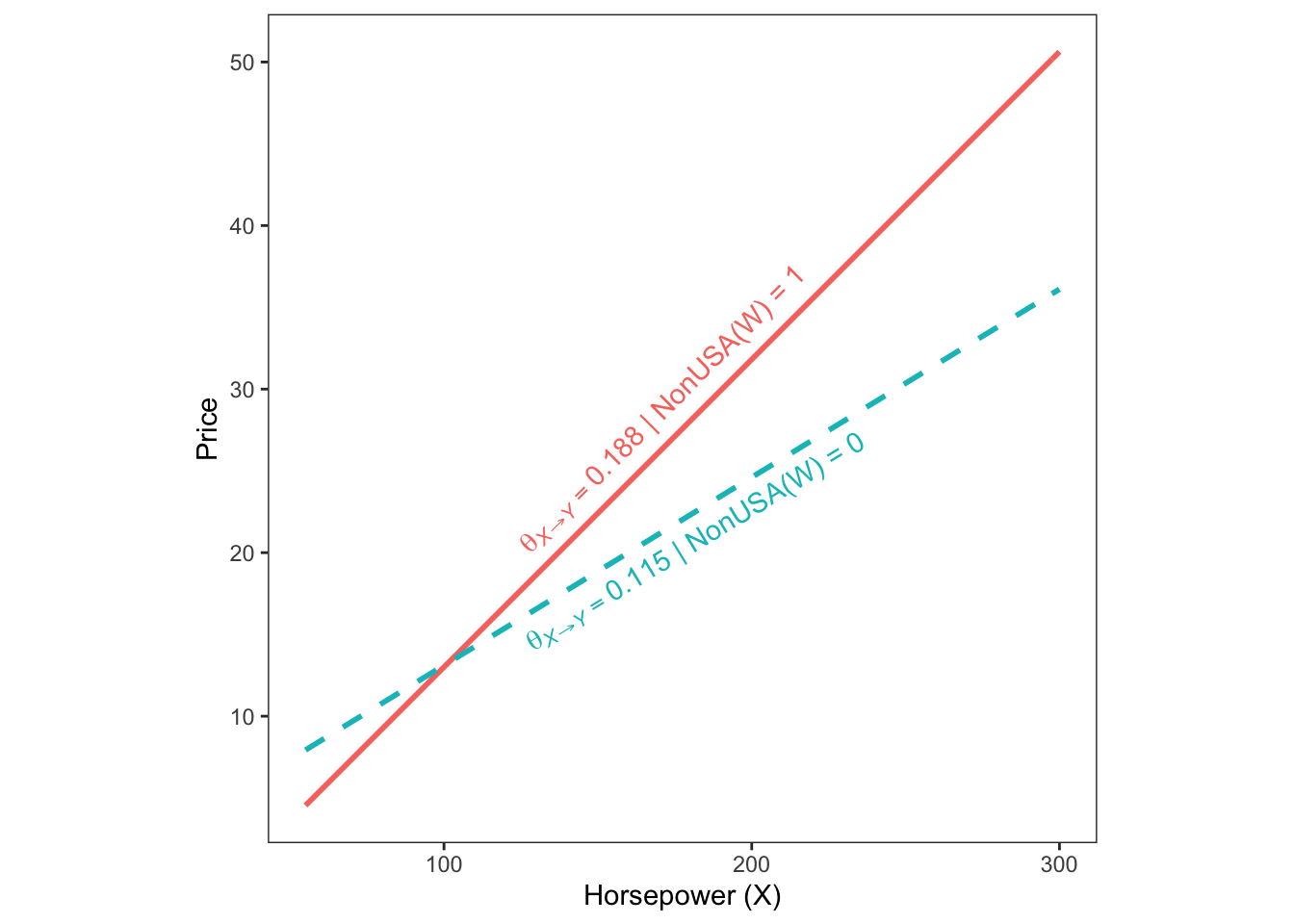

• 그래프를 보면, 제조국에 따라 기울기의 차이가 있음을 알 수 있고, 제조국이 미국이 아닌 경우, Horsepower와 Price의 정적 관계가 더 강함을 볼 수 있습니다.

4.3.2 시내주행연비 조절효과

• 이번에는 시내주행연비의 조절효과를 분석해봅니다.

# 제조국의 조절효과 검증 

fit_lm <- lm(Price~Horsepower*MPG.city,data=data)
labels= list(X="Horsepower",Y="Price",W="MPG.city")
summary(fit_lm)

## 
## Call:
## lm(formula = Price ~ Horsepower * MPG.city, data = data)
## 
## Residuals:
##     Min      1Q  Median      3Q     Max 
## -15.090  -2.775  -0.967   1.655  32.429 
## 
## Coefficients:
##                      Estimate Std. Error t value Pr(>|t|)   
## (Intercept)          0.659343   6.657392   0.099  0.92133   
## Horsepower           0.190782   0.056929   3.351  0.00118 **
## MPG.city             0.075057   0.293089   0.256  0.79847   
## Horsepower:MPG.city -0.003399   0.003095  -1.098  0.27514   
## ---
## Signif. codes:  0 '***' 0.001 '**' 0.01 '*' 0.05 '.' 0.1 ' ' 1
## 
## Residual standard error: 5.943 on 89 degrees of freedom
## Multiple R-squared:  0.6338, Adjusted R-squared:  0.6215 
## F-statistic: 51.35 on 3 and 89 DF,  p-value: < 2.2e-16

modelsSummaryTable(fit_lm,labels = labels)

confint(fit_lm)

##                             2.5 %       97.5 %
## (Intercept)         -12.568753145 13.887440125
## Horsepower            0.077665472  0.303897756
## MPG.city             -0.507305327  0.657419566
## Horsepower:MPG.city  -0.009549485  0.002751554

• 시내주행연비(MPG.city)가 Price에 미치는 영향이 유의하지 않음을 확인할 수 있습니다.
  
• 또한 상호작용항(Horsepower:MPG.city) 역시 유의하지 않음을 확인할 수 있습니다.

4.4 Moderation effect by ProcessR Package

4.4.1 model check

• 두 가설 모두 IV, DV, MO 각각 하나씩만 있기 때문에 Process에서 Model 1번에 해당합니다. 1번 모델 구조와 경로 계수 명칭을 확인합니다.

# 모델 확인
pmacroModel(1)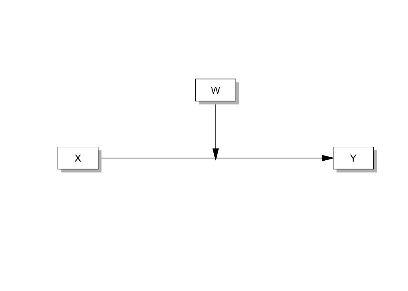

# 모델 경로 계수 명칭 확인
statisticalDiagram(1)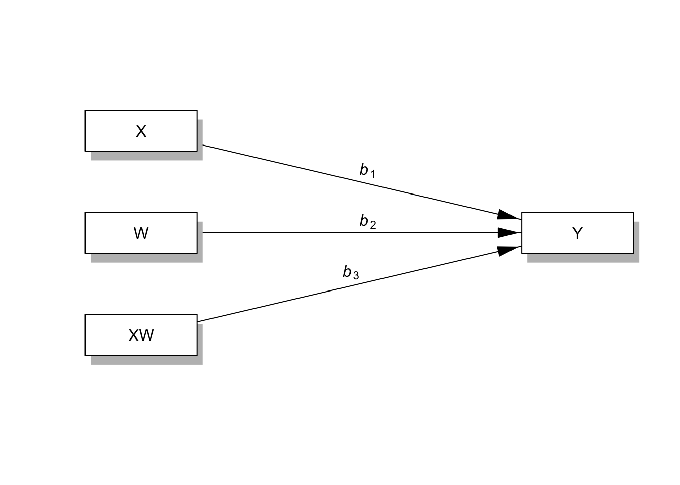 

# b1 : X -> Y
# b2 : W -> Y
# b3 : XW -> Y

4.4.2 model assign : 제조국

• 분석가설에 대해 모델을 설정하고 분석을 진행합니다.

[분석가설] 
  ① 자동차 마력과 자동차 가격 간의 관계에서 자동차 제조국이 조절효과를 할 것이다. 
  
  IV : 자동차 마력(horsepower)
  DV : 자동차 가격(Price)
  Mo : 자동차 제조국

• 이제 모델설정을 해두었으니, 모델방정식을 만들어주면 됩니다.
  
• 독립변인은 Horsepower, 종속변인은 Price, 조절변인은 non-USA입니다.
  
• 회귀분석을 통해 조절효과를 구하면 다음과 같습니다.
  
• ProcessR을 활용하여 그리면 다음과 같습니다.

# 모델 설정 후 그림 그려보기
labels=list(X="Horsepower",W="NonUSA",Y="Price")
pmacroModel(1,labels=labels, radx=0.1,rady=0.07)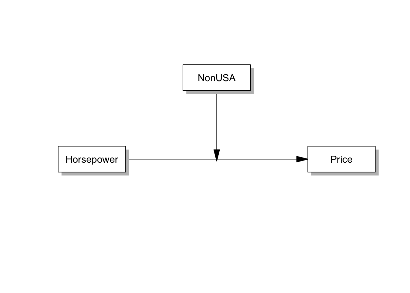

# model equation 만들기 

moderator = list(name="NonUSA", site=list('c'))
model <- modmedEquation(X="Horsepower",Y="Price",labels = labels,moderator = moderator )

# model equation 확인
cat(model)

## 
## Price ~ c1*Horsepower+c2*NonUSA+c3*Horsepower:NonUSA
## NonUSA ~ NonUSA.mean*1
## NonUSA ~~ NonUSA.var*NonUSA

• Moderation Equation이 제대로 설정된 것 같습니다.

• 이제, lavvan 패키지를 활용하여 moderation 분석을 진행하겠습니다.

library(lavaan)

## This is lavaan 0.6-8
## lavaan is FREE software! Please report any bugs.

#bootstrap 200회, msiing value : ml
fit <- sem(model=model,data=data,se='bootstrap',bootstrap=200,missing='ml')

## Warning in lav_partable_vnames(FLAT, "ov.x", warn = TRUE): lavaan WARNING:
##     model syntax contains variance/covariance/intercept formulas
##     involving (an) exogenous variable(s): [NonUSA]; These variables
##     will now be treated as random introducing additional free
##     parameters. If you wish to treat those variables as fixed, remove
##     these formulas from the model syntax. Otherwise, consider adding
##     the fixed.x = FALSE option.

summary(fit,fit.measures = FALSE,standardize = TRUE, rsquare = TRUE)

## lavaan 0.6-8 ended normally after 29 iterations
## 
##   Estimator                                         ML
##   Optimization method                           NLMINB
##   Number of model parameters                         7
##                                                       
##   Number of observations                            93
##   Number of missing patterns                         1
##                                                       
## Model Test User Model:
##                                                       
##   Test statistic                               201.166
##   Degrees of freedom                                 2
##   P-value (Chi-square)                           0.000
## 
## Parameter Estimates:
## 
##   Standard errors                            Bootstrap
##   Number of requested bootstrap draws              200
##   Number of successful bootstrap draws             200
## 
## Regressions:
##                    Estimate  Std.Err  z-value  P(>|z|)   Std.lv  Std.all
##   Price ~                                                               
##     Horsepowr (c1)    0.115    0.015    7.681    0.000    0.115    0.532
##     NonUSA    (c2)   -7.413    3.481   -2.130    0.033   -7.413   -0.329
##     Hrsp:NUSA (c3)    0.073    0.030    2.468    0.014    0.073    0.506
## 
## Intercepts:
##                    Estimate  Std.Err  z-value  P(>|z|)   Std.lv  Std.all
##     NonUSA  (NUSA)    0.484    0.049    9.785    0.000    0.484    0.968
##    .Price             1.607    1.895    0.848    0.397    1.607    0.143
## 
## Variances:
##                    Estimate  Std.Err  z-value  P(>|z|)   Std.lv  Std.all
##     NonUSA  (NUSA)    0.250    0.004   68.185    0.000    0.250    1.000
##    .Price            29.065    7.956    3.653    0.000   29.065    0.229
## 
## R-Square:
##                    Estimate
##     Price             0.771

• 분석 결과 예측변수들을 테이블로 표시할 수 있습니다.

# 모든 파라미터의 Estimates를 표시합니다. 
parameterEstimates(fit,boot.ci.type = 'bca.simple',level = .95, 
ci = TRUE,standardized = FALSE)

## Warning in norm.inter(t, adj.alpha): extreme order statistics used as endpoints

##                  lhs op               rhs       label      est    se      z
## 1              Price  ~        Horsepower          c1    0.115 0.015  7.681
## 2              Price  ~            NonUSA          c2   -7.413 3.481 -2.130
## 3              Price  ~ Horsepower:NonUSA          c3    0.073 0.030  2.468
## 4             NonUSA ~1                   NonUSA.mean    0.484 0.049  9.785
## 5             NonUSA ~~            NonUSA  NonUSA.var    0.250 0.004 68.185
## 6              Price ~~             Price               29.065 7.956  3.653
## 7         Horsepower ~~        Horsepower             2713.583 0.000     NA
## 8         Horsepower ~~ Horsepower:NonUSA              933.807 0.000     NA
## 9  Horsepower:NonUSA ~~ Horsepower:NonUSA             6087.569 0.000     NA
## 10             Price ~1                                  1.607 1.895  0.848
## 11        Horsepower ~1                                143.828 0.000     NA
## 12 Horsepower:NonUSA ~1                                 67.688 0.000     NA
##    pvalue ci.lower ci.upper
## 1   0.000    0.083    0.142
## 2   0.033  -15.036    0.108
## 3   0.014    0.019    0.145
## 4   0.000    0.366    0.581
## 5   0.000    0.249    0.250
## 6   0.000   16.997   55.922
## 7      NA 2713.583 2713.583
## 8      NA  933.807  933.807
## 9      NA 6087.569 6087.569
## 10  0.397   -2.180    5.737
## 11     NA  143.828  143.828
## 12     NA   67.688   67.688

# 논문작성용 테이블을 봅니다. 
estimatesTable2(fit,vanilla = TRUE)

• Bootstrap을 활용한 분석 결과 Horsepower가 Price에 유의미한 정적 영향을 미치고, 제조국에 따른 조절효과가 있음을 알 수 있습니다.

• t 분포가 Z 분포로 변경된 것 외에는 앞서 회귀분석을 통해 구한 지표와 동일합니다.

• 분석 결과를 활용해 아래와 같이 Diagram으로 나타낼 수도 있습니다.

statisticalDiagram(1,labels=labels,fit=fit,whatLabel="est", radx=0.2,rady=0.05)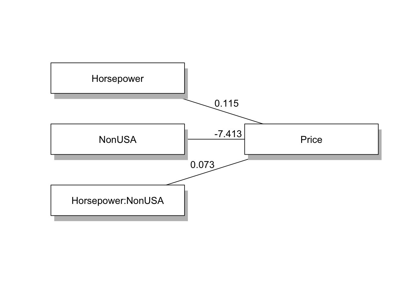

# 변수간 상관계수를 살펴볼 수도 있습니다. 
corTable2(fit)

4.4.3 model assign : 시내주행연비

• 분석가설에 대해 모델을 설정하고 분석을 진행합니다.

[분석가설] 
  ⓶ 자동차 마력과 자동차 가격 간의 관계에서 시내 주행연비가 조절효과를 할 것이다. 
  
  IV : 자동차 마력(horsepower)
  DV : 자동차 가격(Price)
  Mo : 시내 주행연비(MPG.city)

• 이제 모델설정을 해두었으니, 모델방정식을 만들어주면 됩니다.
  
• 독립변인은 Horsepower, 종속변인은 Price, 조절변인은 MPG.city입니다.

# 모델 설정 후 그림 그려보기
labels=list(X="Horsepower",W="MPG.city",Y="Price")
pmacroModel(1,labels=labels, radx=0.1,rady=0.07)

# model equation 만들기 

moderator = list(name="MPG.city", site=list('c'))
model <- modmedEquation(X="Horsepower",Y="Price",labels = labels,moderator = moderator )

# model equation 확인
cat(model)

## 
## Price ~ c1*Horsepower+c2*MPG.city+c3*Horsepower:MPG.city
## MPG.city ~ MPG.city.mean*1
## MPG.city ~~ MPG.city.var*MPG.city

• Moderation Equation이 제대로 설정된 것 같습니다.

• 이제, lavvan 패키지를 활용하여 moderation 분석을 진행하겠습니다.

#bootstrap 200회, msiing value : ml
fit <- sem(model=model,data=data,se='bootstrap',bootstrap=200,missing='ml')

## Warning in lav_partable_vnames(FLAT, "ov.x", warn = TRUE): lavaan WARNING:
##     model syntax contains variance/covariance/intercept formulas
##     involving (an) exogenous variable(s): [MPG.city]; These variables
##     will now be treated as random introducing additional free
##     parameters. If you wish to treat those variables as fixed, remove
##     these formulas from the model syntax. Otherwise, consider adding
##     the fixed.x = FALSE option.

summary(fit,fit.measures = FALSE,standardize = TRUE, rsquare = TRUE)

## lavaan 0.6-8 ended normally after 19 iterations
## 
##   Estimator                                         ML
##   Optimization method                           NLMINB
##   Number of model parameters                         7
##                                                       
##   Number of observations                            93
##   Number of missing patterns                         1
##                                                       
## Model Test User Model:
##                                                       
##   Test statistic                               181.855
##   Degrees of freedom                                 2
##   P-value (Chi-square)                           0.000
## 
## Parameter Estimates:
## 
##   Standard errors                            Bootstrap
##   Number of requested bootstrap draws              200
##   Number of successful bootstrap draws             200
## 
## Regressions:
##                    Estimate    Std.Err  z-value  P(>|z|)   Std.lv    Std.all
##   Price ~                                                                   
##     Horsepowr (c1)      0.191    0.046    4.173    0.000      0.191    1.007
##     MPG.city  (c2)      0.075    0.211    0.355    0.723      0.075    0.042
##     Hrsp:MPG. (c3)     -0.003    0.002   -1.462    0.144     -0.003   -0.250
## 
## Intercepts:
##                    Estimate    Std.Err  z-value  P(>|z|)   Std.lv    Std.all
##     MPG.cty (MPG.)     22.366    0.598   37.390    0.000     22.366    4.001
##    .Price               0.659    5.987    0.110    0.912      0.659    0.067
## 
## Variances:
##                    Estimate    Std.Err  z-value  P(>|z|)   Std.lv    Std.all
##     MPG.cty (MPG.)     31.243    7.598    4.112    0.000     31.243    1.000
##    .Price              33.799   11.372    2.972    0.003     33.799    0.347
## 
## R-Square:
##                    Estimate  
##     Price               0.653

• 분석 결과 예측변수들을 테이블로 표시할 수 있습니다.

# 모든 파라미터의 Estimates를 표시합니다. 
parameterEstimates(fit,boot.ci.type = 'bca.simple',level = .95, 
ci = TRUE,standardized = FALSE)

##                    lhs op                 rhs         label        est     se
## 1                Price  ~          Horsepower            c1      0.191  0.046
## 2                Price  ~            MPG.city            c2      0.075  0.211
## 3                Price  ~ Horsepower:MPG.city            c3     -0.003  0.002
## 4             MPG.city ~1                     MPG.city.mean     22.366  0.598
## 5             MPG.city ~~            MPG.city  MPG.city.var     31.243  7.598
## 6                Price ~~               Price                   33.799 11.372
## 7           Horsepower ~~          Horsepower                 2713.583  0.000
## 8           Horsepower ~~ Horsepower:MPG.city                31928.786  0.000
## 9  Horsepower:MPG.city ~~ Horsepower:MPG.city               529054.266  0.000
## 10               Price ~1                                        0.659  5.987
## 11          Horsepower ~1                                      143.828  0.000
## 12 Horsepower:MPG.city ~1                                     3020.946  0.000
##         z pvalue   ci.lower   ci.upper
## 1   4.173  0.000      0.093      0.277
## 2   0.355  0.723     -0.420      0.443
## 3  -1.462  0.144     -0.007      0.002
## 4  37.390  0.000     21.224     23.577
## 5   4.112  0.000     17.080     47.342
## 6   2.972  0.003     16.881     66.060
## 7      NA     NA   2713.583   2713.583
## 8      NA     NA  31928.786  31928.786
## 9      NA     NA 529054.266 529054.266
## 10  0.110  0.912    -11.322     13.461
## 11     NA     NA    143.828    143.828
## 12     NA     NA   3020.946   3020.946

# 논문작성용 테이블을 봅니다. 
estimatesTable2(fit,vanilla = TRUE)

• Bootstrap을 활용한 분석 결과 Horsepower가 Price에 유의미한 정적 영향을 미치지만, MPG.city는 가격에 유의미한 영향을 미치지 않았습니다.
  

• 또한, MPG.city의 상호작용 효과역시 유의미하지 않았습니다.

• 분석 결과를 Diagram으로 나타내보면, Horsepower를 제외하고는 모두 유의미하지 않음을 알 수 있습니다.

statisticalDiagram(1,labels=labels,fit=fit,whatLabel="est", radx=0.2,rady=0.05)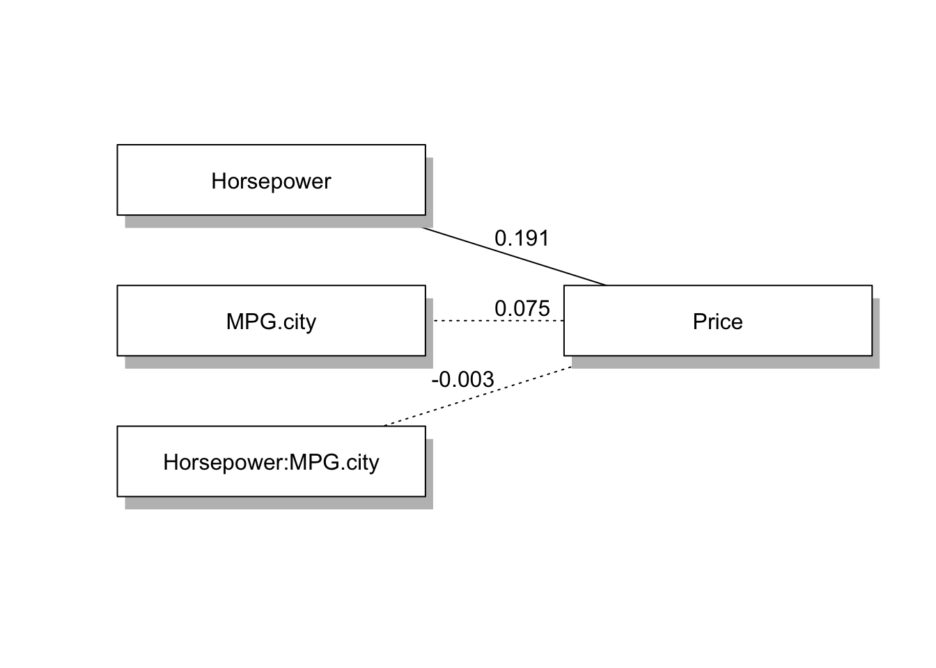

4.5 최종 결과

• 분석결과는 아래와 같습니다.

  
[분석결과] 
  ① 자동차 마력과 자동차 가격 간의 관계에서 자동차 제조국이 조절효과를 할 것이다. 
   -> 채택됨
  ② 자동차 마력과 자동차 가격 간의 관계에서 시내 주행연비가 조절효과를 할 것이다. 
   -> 기각됨