Chapter 5 Conditional Process Analysis

5.1 Data Import

이번 과제에서 활용할 패키지를 불러옵니다.
분석에 사용할 데이터를 복사-붙여넣기 하여 R에서 쉽게 활용할 수 있는 RDS파일로 만들어줍니다.

# 엑셀을 열어 복사하고, data4 변수로 만들어줍니다. 
# 윈도우의 경우, pipe("pbcopy") 대신 "clipboard"를 넣으시면 됩니다. 
# data4 <- read.table(pipe("pbcopy"), sep = '\t', header = TRUE)

# 향후 반복해서 사용하실 수 있도록 RDS 파일로 만들어줍니다. 
# saveRDS(data4,"data4.RDS")

여러가지 변수들이 있지만, 제가 오늘 사용할 변수는 아래와 같습니다.
- presence of calling (T2)
- Transformational Leadership(T2)
- Person-Job Fit(T2)
- Job Satisfaction(T2)
보다 편리한 분석을 위해 data4에서 필요한 변수들만 가지고
별도의 데이터 프레임을 구성합니다.

data4 <- readRDS("data4.RDS")
data4%>%select(V1, ID, T1sex,T1age, T1edu, T1religion, email, Company, 
               T2소명P,  T2leadership,  T2PJfit, T2JS, T2소명P1, T2소명P2,
               T2소명P3R, T2소명P4,T2소명P5,T2소명P6,T2소명P7,T2소명P8,T2소명P9,
               T2소명P10,T2소명P11,T2소명P12, T2leadership1,T2leadership2,T2leadership3,
               T2leadership4,T2leadership5,T2leadership6,T2leadership7, T2PJfit1,
               T2PJfit2,T2PJfiT2_A,T2PJfit4,T2PJfit5, T2JS1,T2JS2R,T2JS3,T2JS4,T2JS4,T2JS5,
               T2JS6)->raw_data

str(raw_data)

## 'data.frame':    151 obs. of  42 variables:
##  $ V1           : int  1 2 3 4 5 6 7 8 9 10 ...
##  $ ID           : int  18 542 316 370 421 498 549 205 436 50 ...
##  $ T1sex        : int  1 1 1 2 2 1 1 1 1 1 ...
##  $ T1age        : int  30 25 27 24 24 26 25 25 26 25 ...
##  $ T1edu        : int  4 3 3 3 3 3 3 3 3 3 ...
##  $ T1religion   : int  3 1 1 1 1 1 4 1 4 4 ...
##  $ email        : chr  "bj.juhng" "bk.jin" "bo.kim" "bomiu.park" ...
##  $ Company      : int  4 6 5 7 6 5 6 5 6 6 ...
##  $ T2소명P      : num  3 2.92 3.17 3.67 2.5 ...
##  $ T2leadership : num  4 4.14 4 4.14 3.43 ...
##  $ T2PJfit      : num  5 5 6 5.4 4 5.4 5 3.8 6 5 ...
##  $ T2JS         : num  4 4 4.17 4.17 3.67 ...
##  $ T2소명P1     : int  3 3 3 4 2 2 4 1 4 4 ...
##  $ T2소명P2     : int  4 4 4 5 3 4 4 1 4 4 ...
##  $ T2소명P3R    : int  2 3 2 2 2 1 2 2 2 2 ...
##  $ T2소명P4     : int  3 3 3 4 2 4 3 2 3 4 ...
##  $ T2소명P5     : int  2 1 2 2 2 1 3 2 2 3 ...
##  $ T2소명P6     : int  3 3 4 4 2 4 3 2 2 3 ...
##  $ T2소명P7     : int  3 4 3 5 3 5 4 2 4 4 ...
##  $ T2소명P8     : int  3 4 4 3 3 4 4 2 4 5 ...
##  $ T2소명P9     : int  4 4 4 4 4 5 4 3 4 5 ...
##  $ T2소명P10    : int  3 3 3 4 2 4 3 2 4 5 ...
##  $ T2소명P11    : int  2 1 2 2 2 2 3 1 2 4 ...
##  $ T2소명P12    : int  4 4 4 5 3 5 3 3 4 4 ...
##  $ T2leadership1: int  4 4 4 4 4 2 3 2 4 3 ...
##  $ T2leadership2: int  4 4 4 4 3 2 4 2 4 4 ...
##  $ T2leadership3: int  4 4 4 4 3 2 4 2 4 3 ...
##  $ T2leadership4: int  4 4 4 4 4 5 4 3 4 5 ...
##  $ T2leadership5: int  4 4 4 4 3 4 3 2 4 4 ...
##  $ T2leadership6: int  4 5 4 4 4 5 4 2 4 4 ...
##  $ T2leadership7: int  4 4 4 5 3 2 4 2 4 3 ...
##  $ T2PJfit1     : int  5 5 6 5 4 5 5 7 6 5 ...
##  $ T2PJfit2     : int  5 5 6 6 4 6 4 6 6 4 ...
##  $ T2PJfiT2_A   : int  5 5 6 5 4 5 4 3 6 4 ...
##  $ T2PJfit4     : int  5 5 6 6 4 5 6 2 6 6 ...
##  $ T2PJfit5     : int  5 5 6 5 4 6 6 1 6 6 ...
##  $ T2JS1        : int  4 4 4 4 4 4 4 1 4 5 ...
##  $ T2JS2R       : int  4 4 5 5 4 4 4 2 5 5 ...
##  $ T2JS3        : int  4 4 4 4 4 1 4 2 4 5 ...
##  $ T2JS4        : int  4 4 4 4 4 2 4 2 4 5 ...
##  $ T2JS5        : int  4 4 4 4 3 5 3 2 4 4 ...
##  $ T2JS6        : int  4 4 4 4 3 2 3 1 4 4 ...

5.2 Descriptive analysis

5.2.1 연구대상자 특성

필요한 데이터들만 정리했으니, 먼저 연구 대상자의 특성을 살펴보겠습니다.
성별에 따른 특성을 살펴보면 아래와 같습니다.

 raw_data%>%select(Company,T1sex,T1age, T1edu, T1religion)-> descriptive
  mytable(T1sex~., data=descriptive)->res
  myhtml(res, caption=paste0("Table1. 연구대상자의 일반적 특성"))

Table1. 연구대상자의 일반적 특성
T1sex	1 (N=109)	2 (N=42)	p
Company	4.7 ± 1.7	4.6 ± 1.7	0.776
T1age	25.7 ± 1.4	23.4 ± 1.5	0.000
T1edu			0.223
3	102 (93.6%)	36 (85.7%)
4	7 ( 6.4%)	6 (14.3%)
T1religion			0.877
1	67 (61.5%)	26 (61.9%)
2	17 (15.6%)	7 (16.7%)
3	10 ( 9.2%)	5 (11.9%)
4	15 (13.8%)	4 ( 9.5%)

성별은 남자가 109명, 여자가 42명으로 남자가 좀 더 많았고, 나이는 남성 편균은 25.7세, 여성 평균은 23.4세 였습니다.
학력 수준은 학사 출신이 총 138명, 석사가 13명이었습니다.
종교는 종교없음 93명, 개신교 24명, 천주교 15명, 불교가 19명입니다.

5.2.2 측정변수 기술통계

이제, 측정변수를 계산한 뒤, 기술통계를 살펴보겠습니다.
상관관계를 확인하기 위해, corstars 함수를 정의합니다.

corstars <-function(x, method=c("pearson", "spearman"), removeTriangle=c("upper", "lower"), result=c("none", "html", "latex")){
    #Compute correlation matrix
    require(Hmisc)
    x <- as.matrix(x)
    correlation_matrix<-rcorr(x, type=method[1])
    R <- correlation_matrix$r # Matrix of correlation coeficients
    p <- correlation_matrix$P # Matrix of p-value 
    
    ## Define notions for significance levels; spacing is important.
    mystars <- ifelse(p < .0001, "****", ifelse(p < .001, "*** ", ifelse(p < .01, "**  ", ifelse(p < .05, "*   ", "    "))))
    
    ## trunctuate the correlation matrix to two decimal
    R <- format(round(cbind(rep(-1.11, ncol(x)), R), 2))[,-1]
    
    ## build a new matrix that includes the correlations with their apropriate stars
    Rnew <- matrix(paste(R, mystars, sep=""), ncol=ncol(x))
    diag(Rnew) <- paste(diag(R), " ", sep="")
    rownames(Rnew) <- colnames(x)
    colnames(Rnew) <- paste(colnames(x), "", sep="")
    
    ## remove upper triangle of correlation matrix
    if(removeTriangle[1]=="upper"){
      Rnew <- as.matrix(Rnew)
      Rnew[upper.tri(Rnew, diag = TRUE)] <- ""
      Rnew <- as.data.frame(Rnew)
    }
    
    ## remove lower triangle of correlation matrix
    else if(removeTriangle[1]=="lower"){
      Rnew <- as.matrix(Rnew)
      Rnew[lower.tri(Rnew, diag = TRUE)] <- ""
      Rnew <- as.data.frame(Rnew)
    }
    
    ## remove last column and return the correlation matrix
    Rnew <- cbind(Rnew[1:length(Rnew)-1])
    if (result[1]=="none") return(Rnew)
    else{
      if(result[1]=="html") print(xtable(Rnew), type="html")
      else print(xtable(Rnew), type="latex") 
    }
}

소명(Calling), 직무몰입(Job Involvement), 인지된 조직지지(Perceived organizational support), 잡크래프팅(Job Crafting) 변수에 대한 상관 및 표준편차는 다음과 같습니다.

# 기술통계를 위한 변수 상관 구하기 : 유의성까지 포함해서 표로 보기 
raw_data%>%select(T2소명P,  T2leadership,  T2PJfit, T2JS)%>%
  reshape::rename(c(T2소명P='presence_of_calling', T2leadership='Trans_leadership',
                    T2PJfit='Person_Job_fit', T2JS="Job_Satisfaction"))%>%corstars(method="pearson", result="html")

	presence_of_calling	Trans_leadership	Person_Job_fit
presence_of_calling
Trans_leadership	0.29***
Person_Job_fit	0.33****	0.43****
Job_Satisfaction	0.41****	0.61****	0.61****

# 평균 및 표준편차 
raw_data%>%select(T2소명P,  T2leadership,  T2PJfit, T2JS)%>%
  reshape::rename(c(T2소명P='presence_of_calling', T2leadership='Trans_leadership',
                    T2PJfit='Person_Job_fit', T2JS="Job_Satisfaction"))%>%
  stargazer(title='Descriptive statistics', digits = 2, type = "html", 
            out = "desc_4.html", summary.stat = c("n", "mean", "sd", "median", "min", "max"))

**Descriptive statistics**

Statistic	N	Mean	St. Dev.	Median	Min	Max

presence_of_calling	151	3.27	0.63	3.2	1	5
Trans_leadership	151	3.79	0.72	4	1	5
Person_Job_fit	151	4.85	0.98	5	1	7
Job_Satisfaction	151	3.59	0.73	3.7	2	5

기술통계 결과를 보면, 네 가지 요인이 모두 유의미한 정적 상관을 보이고 있으며,
perceived organizational support와 Job Crafting 간의 상관 관계가 가장 높게 나타났습니다.
Perceived organizational support와 search for calling 간 상관은 유의미하지 않는 것으로 나타났으나, 조절변수는 이론적으로 설정하는 것이기 때문에

5.3 신뢰도 분석

# T2 presence of calling 신뢰도 분석
raw_data%>%select(T2소명P1, T2소명P2,
               T2소명P3R, T2소명P4,T2소명P5,T2소명P6,T2소명P7,T2소명P8,T2소명P9,
               T2소명P10,T2소명P11,T2소명P12)%>%alpha()

## 
## Reliability analysis   
## Call: alpha(x = .)
## 
##   raw_alpha std.alpha G6(smc) average_r S/N   ase mean   sd median_r
##       0.88      0.88    0.91      0.38 7.5 0.015  3.3 0.63      0.4
## 
##  lower alpha upper     95% confidence boundaries
## 0.85 0.88 0.9 
## 
##  Reliability if an item is dropped:
##           raw_alpha std.alpha G6(smc) average_r S/N alpha se var.r med.r
## T2소명P1       0.86      0.87    0.89      0.37 6.5    0.017 0.034  0.39
## T2소명P2       0.87      0.88    0.90      0.40 7.4    0.015 0.031  0.42
## T2소명P3R      0.89      0.89    0.91      0.43 8.3    0.013 0.017  0.42
## T2소명P4       0.87      0.87    0.90      0.38 6.9    0.016 0.031  0.40
## T2소명P5       0.87      0.87    0.90      0.39 7.0    0.016 0.032  0.40
## T2소명P6       0.86      0.87    0.89      0.37 6.5    0.017 0.032  0.39
## T2소명P7       0.86      0.87    0.89      0.37 6.6    0.016 0.029  0.38
## T2소명P8       0.87      0.88    0.90      0.40 7.3    0.015 0.030  0.40
## T2소명P9       0.87      0.87    0.90      0.39 7.0    0.015 0.031  0.41
## T2소명P10      0.86      0.86    0.89      0.37 6.4    0.017 0.030  0.38
## T2소명P11      0.86      0.87    0.89      0.37 6.4    0.017 0.031  0.39
## T2소명P12      0.86      0.86    0.88      0.36 6.2    0.017 0.028  0.38
## 
##  Item statistics 
##             n raw.r std.r r.cor r.drop mean   sd
## T2소명P1  151  0.75  0.74  0.72   0.68  3.1 1.01
## T2소명P2  151  0.51  0.54  0.47   0.42  3.7 0.85
## T2소명P3R 151  0.39  0.34  0.27   0.24  2.6 1.17
## T2소명P4  151  0.65  0.66  0.62   0.57  3.1 0.98
## T2소명P5  151  0.67  0.63  0.59   0.57  2.5 1.14
## T2소명P6  151  0.76  0.75  0.72   0.69  3.2 1.02
## T2소명P7  151  0.69  0.72  0.71   0.63  3.7 0.82
## T2소명P8  151  0.53  0.56  0.50   0.44  3.5 0.88
## T2소명P9  151  0.59  0.63  0.59   0.52  4.0 0.71
## T2소명P10 151  0.78  0.78  0.77   0.71  3.3 0.99
## T2소명P11 151  0.80  0.76  0.75   0.73  2.7 1.19
## T2소명P12 151  0.79  0.82  0.82   0.74  3.8 0.80
## 
## Non missing response frequency for each item
##              1    2    3    4    5 miss
## T2소명P1  0.07 0.19 0.36 0.32 0.05    0
## T2소명P2  0.02 0.05 0.27 0.51 0.15    0
## T2소명P3R 0.19 0.30 0.24 0.21 0.05    0
## T2소명P4  0.01 0.29 0.38 0.21 0.10    0
## T2소명P5  0.21 0.34 0.26 0.13 0.06    0
## T2소명P6  0.04 0.23 0.32 0.32 0.09    0
## T2소명P7  0.01 0.06 0.28 0.50 0.16    0
## T2소명P8  0.01 0.11 0.40 0.36 0.13    0
## T2소명P9  0.01 0.01 0.19 0.57 0.23    0
## T2소명P10 0.04 0.16 0.38 0.32 0.11    0
## T2소명P11 0.18 0.28 0.28 0.18 0.08    0
## T2소명P12 0.01 0.04 0.26 0.51 0.19    0

# raw_alpha 0.88로 0.7 이상으로 나타남
# 모든 문항이 .8 이상으로 양호함

# T2 Transformational leadership 신뢰도 분석
raw_data%>%select(T2leadership1,T2leadership2,T2leadership3,
               T2leadership4,T2leadership5,T2leadership6,T2leadership7)%>%alpha()

## 
## Reliability analysis   
## Call: alpha(x = .)
## 
##   raw_alpha std.alpha G6(smc) average_r S/N  ase mean   sd median_r
##       0.92      0.92    0.92      0.62  12 0.01  3.8 0.72     0.62
## 
##  lower alpha upper     95% confidence boundaries
## 0.9 0.92 0.94 
## 
##  Reliability if an item is dropped:
##               raw_alpha std.alpha G6(smc) average_r  S/N alpha se  var.r med.r
## T2leadership1      0.91      0.91    0.91      0.62  9.9    0.012 0.0094  0.62
## T2leadership2      0.90      0.91    0.90      0.61  9.5    0.012 0.0056  0.62
## T2leadership3      0.90      0.90    0.89      0.60  9.1    0.013 0.0026  0.61
## T2leadership4      0.91      0.91    0.91      0.63 10.1    0.012 0.0084  0.62
## T2leadership5      0.91      0.91    0.91      0.62  9.9    0.012 0.0093  0.62
## T2leadership6      0.92      0.92    0.91      0.65 11.4    0.010 0.0043  0.63
## T2leadership7      0.90      0.91    0.90      0.61  9.6    0.012 0.0061  0.62
## 
##  Item statistics 
##                 n raw.r std.r r.cor r.drop mean   sd
## T2leadership1 151  0.82  0.82  0.78   0.75  3.6 0.88
## T2leadership2 151  0.84  0.84  0.82   0.78  3.9 0.84
## T2leadership3 151  0.87  0.88  0.87   0.82  3.8 0.85
## T2leadership4 151  0.81  0.81  0.76   0.73  3.8 0.87
## T2leadership5 151  0.82  0.82  0.78   0.75  3.7 0.88
## T2leadership6 151  0.74  0.74  0.68   0.64  4.0 0.91
## T2leadership7 151  0.85  0.84  0.82   0.78  3.7 0.92
## 
## Non missing response frequency for each item
##                  1    2    3    4    5 miss
## T2leadership1 0.02 0.10 0.23 0.54 0.11    0
## T2leadership2 0.01 0.05 0.17 0.54 0.24    0
## T2leadership3 0.01 0.07 0.20 0.56 0.16    0
## T2leadership4 0.01 0.08 0.19 0.54 0.17    0
## T2leadership5 0.01 0.09 0.26 0.47 0.17    0
## T2leadership6 0.01 0.06 0.15 0.46 0.32    0
## T2leadership7 0.01 0.09 0.25 0.46 0.19    0

# raw_alpha 0.9로 높게 나타남
# 모든 문항이 .8 이상으로 양호함

# T2 person-job fit 신뢰도 분석
raw_data%>%select(T2PJfit1,
               T2PJfit2,T2PJfiT2_A,T2PJfit4,T2PJfit5)%>%alpha()

## 
## Reliability analysis   
## Call: alpha(x = .)
## 
##   raw_alpha std.alpha G6(smc) average_r S/N   ase mean   sd median_r
##       0.89      0.89    0.92      0.62 8.2 0.015  4.9 0.98     0.63
## 
##  lower alpha upper     95% confidence boundaries
## 0.86 0.89 0.92 
## 
##  Reliability if an item is dropped:
##            raw_alpha std.alpha G6(smc) average_r S/N alpha se var.r med.r
## T2PJfit1        0.87      0.87    0.89      0.63 6.7    0.018 0.024  0.63
## T2PJfit2        0.87      0.87    0.88      0.63 6.7    0.018 0.020  0.63
## T2PJfiT2_A      0.85      0.85    0.89      0.59 5.7    0.022 0.033  0.50
## T2PJfit4        0.88      0.88    0.87      0.65 7.4    0.016 0.016  0.68
## T2PJfit5        0.86      0.87    0.86      0.62 6.4    0.019 0.022  0.64
## 
##  Item statistics 
##              n raw.r std.r r.cor r.drop mean  sd
## T2PJfit1   151  0.82  0.83  0.78   0.72  5.0 1.1
## T2PJfit2   151  0.82  0.83  0.79   0.71  4.7 1.2
## T2PJfiT2_A 151  0.88  0.88  0.85   0.81  4.5 1.1
## T2PJfit4   151  0.80  0.79  0.76   0.68  5.0 1.3
## T2PJfit5   151  0.85  0.84  0.82   0.75  5.0 1.2
## 
## Non missing response frequency for each item
##               1    2    3    4    5    6    7 miss
## T2PJfit1   0.01 0.01 0.04 0.27 0.36 0.22 0.10    0
## T2PJfit2   0.01 0.02 0.14 0.25 0.35 0.18 0.06    0
## T2PJfiT2_A 0.01 0.03 0.13 0.32 0.30 0.18 0.03    0
## T2PJfit4   0.00 0.05 0.08 0.15 0.32 0.30 0.09    0
## T2PJfit5   0.01 0.02 0.09 0.20 0.32 0.29 0.07    0

# raw_alpha 0.89로 높게 나타남
# 모든 문항이 .7 이상으로 양호함

# T2 job satisfaction에 대해 신뢰도 분석을 다시 하고, 
raw_data%>%select(T2JS1,T2JS2R,T2JS3,T2JS4,T2JS4,T2JS5,T2JS6)%>%alpha()

## 
## Reliability analysis   
## Call: alpha(x = .)
## 
##   raw_alpha std.alpha G6(smc) average_r S/N   ase mean   sd median_r
##       0.88      0.88    0.89      0.56 7.6 0.016  3.6 0.73      0.6
## 
##  lower alpha upper     95% confidence boundaries
## 0.85 0.88 0.91 
## 
##  Reliability if an item is dropped:
##        raw_alpha std.alpha G6(smc) average_r S/N alpha se  var.r med.r
## T2JS1       0.84      0.85    0.85      0.52 5.5    0.021 0.0283  0.55
## T2JS2R      0.90      0.90    0.90      0.64 9.0    0.013 0.0065  0.65
## T2JS3       0.85      0.86    0.85      0.54 6.0    0.020 0.0237  0.59
## T2JS4       0.84      0.84    0.85      0.52 5.4    0.021 0.0215  0.56
## T2JS5       0.86      0.86    0.86      0.56 6.4    0.019 0.0249  0.59
## T2JS6       0.86      0.86    0.86      0.56 6.3    0.019 0.0221  0.57
## 
##  Item statistics 
##          n raw.r std.r r.cor r.drop mean   sd
## T2JS1  151  0.87  0.87  0.84   0.80  3.7 0.95
## T2JS2R 151  0.64  0.62  0.50   0.46  3.9 1.02
## T2JS3  151  0.82  0.83  0.80   0.73  3.6 0.83
## T2JS4  151  0.87  0.87  0.86   0.80  3.7 0.87
## T2JS5  151  0.79  0.79  0.75   0.69  3.4 0.93
## T2JS6  151  0.79  0.79  0.75   0.69  3.3 0.93
## 
## Non missing response frequency for each item
##           1    2    3    4    5 miss
## T2JS1  0.01 0.13 0.19 0.50 0.17    0
## T2JS2R 0.02 0.10 0.17 0.40 0.30    0
## T2JS3  0.01 0.09 0.26 0.54 0.10    0
## T2JS4  0.01 0.08 0.26 0.50 0.15    0
## T2JS5  0.02 0.15 0.31 0.42 0.10    0
## T2JS6  0.03 0.18 0.34 0.38 0.07    0

# raw_alpha 0.87로 높게 나타남
# 모든 문항이 .9 이상으로 양호함

5.4 Moderating effect analysis

5.4.1 조절효과 분석

조절된 매개효과를 분석하기에 앞서, 조절효과와 매개효과를 분석해줍니다.

reshape::rename(raw_data,c(T2소명P='presence_of_calling', T2leadership='Trans_leadership',
                    T2PJfit='Person_Job_fit', T2JS="Job_Satisfaction"))->raw_data
labels=list(X='presence_of_calling', Y="Job_Satisfaction", W='Person_Job_fit')
pmacroModel(1, labels = labels, radx=0.15,rady=0.05)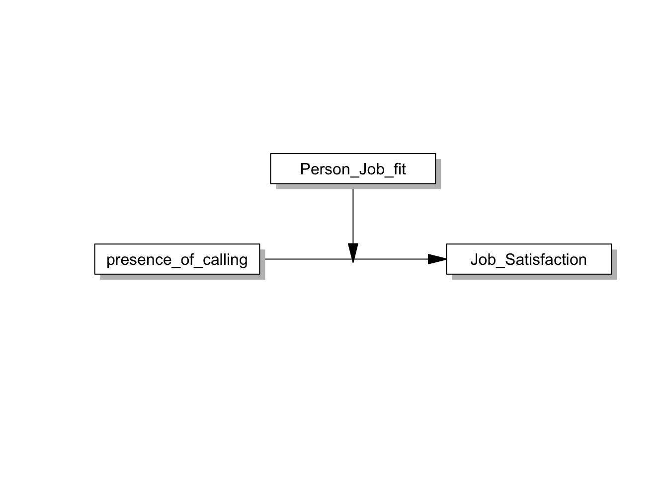

위와 같이 모델 설정 후, 회귀분석을 활용하여 분석합니다.

fit <- lm(Job_Satisfaction ~ presence_of_calling*Person_Job_fit, raw_data)

modelsSummaryTable(fit, labels=labels)

	Consequent
presence_of_calling(X)	c1	0.326	0.330	0.986	.326
Person_Job_fit(W)	c2	0.433	0.210	2.061	.041
presence_of_calling:Person_Job_fit(X:W)	c3	-0.011	0.062	-0.175	.862
Constant	iY	0.602	1.079	0.558	.578
Observations		151
R2		0.423
Adjusted R2		0.411
Residual SE		0.560 ( df = 147)
F statistic		F(3,147) = 35.907, p < .001

조절효과의 회귀계수는 -0.011이며, 통계적으로 유의하지 않은 것으로 나타났습니다.

5.5 매개효과 분석

매개효과는 다음과 같은 모델을 설정하여 분석합니다.

labels=list(X='presence_of_calling', Y="Job_Satisfaction", M='Trans_leadership')

statisticalDiagram(4,labels = labels,radx=0.15,rady=0.05)

- 이 모형을 분석하면 다음과 같습니다.

result <- mediationBK(labels=labels, data=raw_data)

modelsSummaryTable(result$fit, labels=labels)

	Consequent
presence_of_calling(X)	c	0.471	0.086	5.476	<.001	a	0.331	0.089	3.698	<.001	c'	0.293	0.075	3.921	<.001
Trans_leadership(M)											b	0.538	0.066	8.209	<.001
Constant	iY	2.051	0.287	7.151	<.001	iM	2.711	0.298	9.098	<.001	iY	0.591	0.297	1.988	.049
Observations		151			151		151
R2		0.168			0.084		0.428
Adjusted R2		0.162			0.078		0.420
Residual SE		0.668 ( df = 149)			0.694 ( df = 149)		0.555 ( df = 148)
F statistic		F(1,149) = 29.986, p < .001			F(1,149) = 13.674, p < .001		F(2,148) = 55.364, p < .001

분석결과를 통계적 모형으로 나타내면 다음과 같습니다.

plot(result, type=1, ylim=c(0.3, 0.6))

plot(result)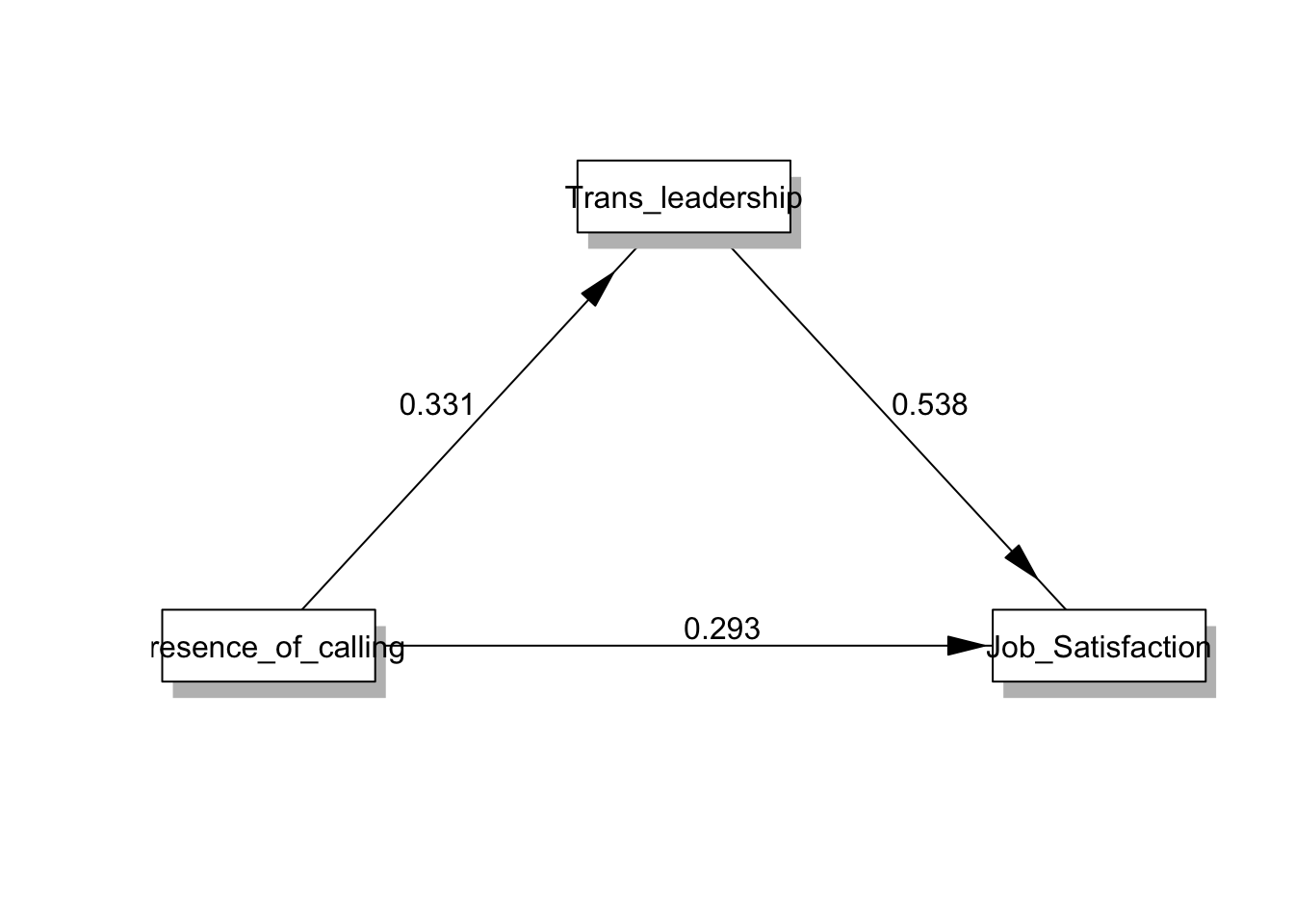

매개 모형의 간접효과를 부투스트래핑 방법으로 구하기 위해 laavan 패키지를 활용합니다.

model <- tripleEquation(labels=labels, data = raw_data)

set.seed(123)
semfit <- sem(model = model, data=raw_data, se="boot")

medSummaryTable(semfit)

Effect	Equation	estimate	95% Bootstrap CI
indirect	(a)*(b)	0.178	(0.053 to 0.326)
direct	c	0.293	(0.103 to 0.486)
total	direct+indirect	0.471	(0.270 to 0.688)
prop.mediated	indirect/total	0.378	(0.128 to 0.709)
boot.ci.type = perc

매개효과 검증 결과 간접효과를 비롯하여 산출된 신뢰구간 내에 0을 포함하고 있지 않으므로 매개효과는 유의합니다.

5.6 Moderated Mediation analysis

5.6.1 모델 설정

조절된 매개 모형(Process Macro Model 8)을 설정해줍니다.

labels <- list(X='presence_of_calling', Y="Job_Satisfaction", W='Person_Job_fit', M='Trans_leadership')
pmacroModel(8, labels=labels, radx=0.13,rady=0.05)

Process Macro Model 8의 통계적 모형은 다음과 같습니다.

statisticalDiagram(8, labels=labels, radx=0.15,rady=0.05)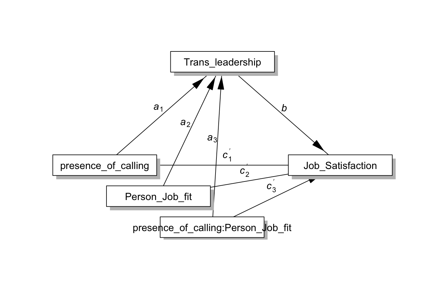

### 회귀분석을 활용한 조절된 매개효과 분석

위 모형을 회귀식으로 설정하면 다음과 같습니다.

moderator <- list(name="Person_Job_fit", site=list(c("a","c")))
equation <- tripleEquation(labels = labels, moderator=moderator, mode=1)
cat(equation)

## Trans_leadership~presence_of_calling+Person_Job_fit+presence_of_calling:Person_Job_fit
## Job_Satisfaction~presence_of_calling+Person_Job_fit+presence_of_calling:Person_Job_fit+Trans_leadership

이제 위의 회귀식을 활용해서 회귀모형의 리스트를 만듭니다.

fit=eq2fit(equation, data=raw_data)

modelsSummary(fit, labels=labels)

## ==================================================================================================== 
##                                                          Consequent                                  
##                          --------------------------------------------------------------------------- 
##                                   Trans_leadership(M)                  Job_Satisfaction(Y)         
##                          -------------------------------------  -------------------------------------  
##        Antecedent               Coef     SE      t       p            Coef     SE      t       p     
## ---------------------------------------------------------------------------------------------------- 
##  presence_of_calling(X)   a1  -0.607   0.377  -1.611    .109  c'1   0.575   0.295   1.949    .053  
##     Person_Job_fit(W)     a2  -0.233   0.240  -0.972    .333  c'2   0.529   0.187   2.831    .005  
## presence_of_calling:Person_Job_fit(X:W) a3   0.155   0.071   2.177    .031  c'3  -0.074   0.056  -1.328    .186  
##    Trans_leadership(M)                                          b   0.411   0.064   6.418   <.001  
##         Constant          iM   4.422   1.232   3.588   <.001   iY  -1.214   0.997  -1.217    .225  
## ---------------------------------------------------------------------------------------------------- 
##       Observations                        151                                  151                 
##            R2                            0.233                                0.550                
##        Adjusted R2                       0.217                                0.538                
##        Residual SE                 0.639 ( df = 147)                    0.496 ( df = 146)          
##        F statistic            F(3,147) = 14.883, p < .001          F(4,146) = 44.591, p < .001     
## ====================================================================================================

조절된 매개모형의 회귀계수는 위와 같다.
회귀분석 결과를 회귀계수를 이용하여 통계적 모형을 그려보면 아래와 같다.

drawModel(fit, labels = labels, whatLabel = 'est', ymargin = .000001, xmargin = .000001, rady = 0.05)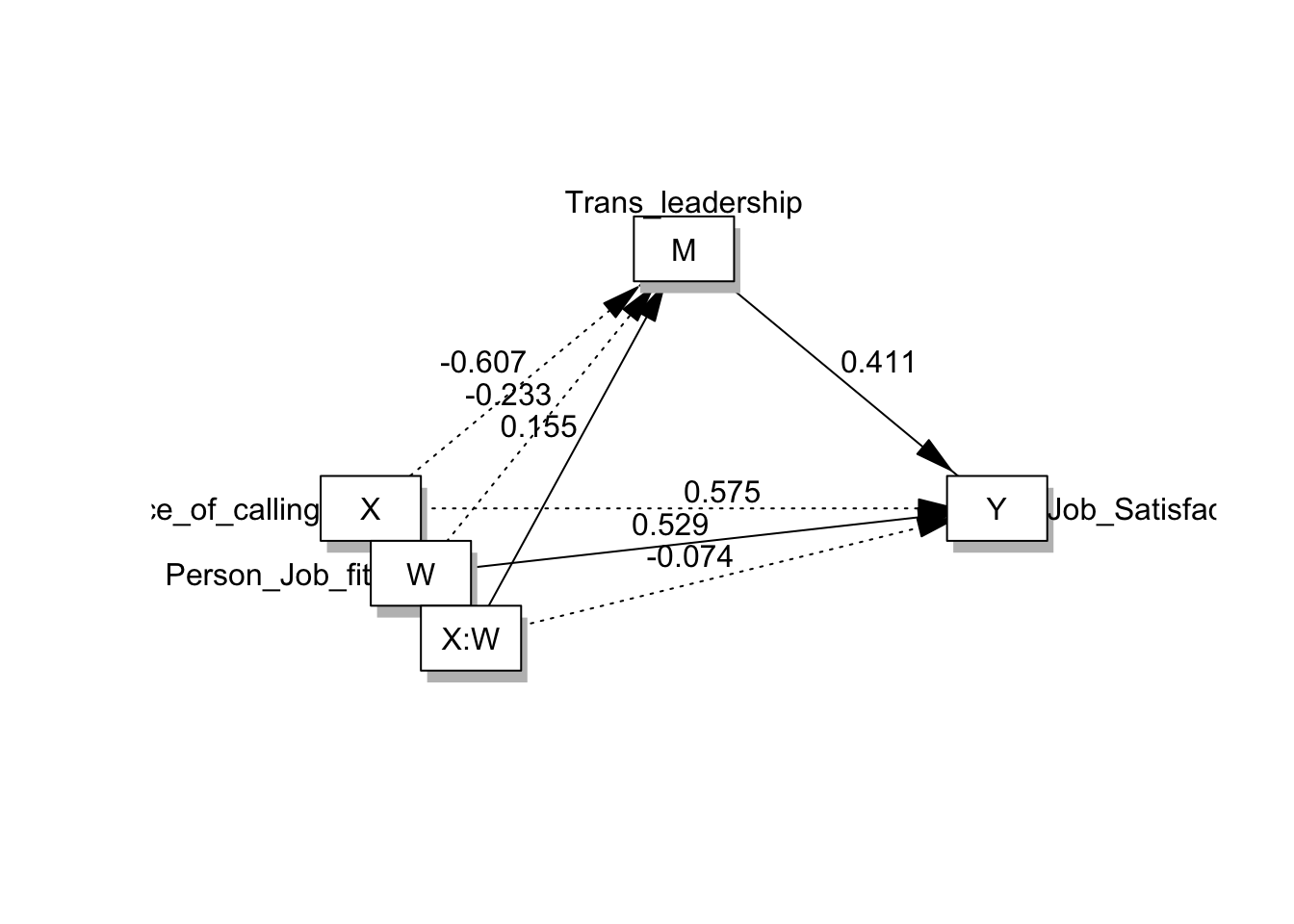

5.6.2 조건부 직접효과와 간접효과의 추정

SEM을 활용하여 부트스트래핑을 하고, 이를 기반으로 신뢰구간을 얻기 위해 SEM syntax를 만들어줍니다.

model=tripleEquation(label=labels, moderator=moderator,rangemode=2, data=raw_data)

cat(model)

## Trans_leadership~a1*presence_of_calling+a2*Person_Job_fit+a3*presence_of_calling:Person_Job_fit
## Job_Satisfaction~c1*presence_of_calling+c2*Person_Job_fit+c3*presence_of_calling:Person_Job_fit+b*Trans_leadership
## Person_Job_fit ~ Person_Job_fit.mean*1
## Person_Job_fit ~~ Person_Job_fit.var*Person_Job_fit
## CE.XonM :=a1+a3*5
## indirect :=(a1+a3*5)*(b)
## index.mod.med :=a3*b
## direct :=c1+c3*5
## total := direct + indirect
## prop.mediated := indirect / total
## CE.XonM.below :=a1+a3*3.8
## indirect.below :=(a1+a3*3.8)*(b)
## CE.XonM.above :=a1+a3*5.8
## indirect.above :=(a1+a3*5.8)*(b)
## direct.below:=c1+c3*3.8
## direct.above:=c1+c3*5.8
## total.below := direct.below + indirect.below
## total.above := direct.above + indirect.above
## prop.mediated.below := indirect.below / total.below
## prop.mediated.above := indirect.above / total.above

이제 이를 토대로 분석을 해보겠습니다.

set.seed(1234)
semfit=sem(model=model,data= raw_data, se="boot")

## Warning in lav_partable_vnames(FLAT, "ov.x", warn = TRUE): lavaan WARNING:
##     model syntax contains variance/covariance/intercept formulas
##     involving (an) exogenous variable(s): [Person_Job_fit]; These
##     variables will now be treated as random introducing additional
##     free parameters. If you wish to treat those variables as fixed,
##     remove these formulas from the model syntax. Otherwise, consider
##     adding the fixed.x = FALSE option.

estimatesTable2(semfit)

Variables	Predictors	label	B	SE	z	p	β
Trans_leadership	presence_of_calling	a1	-0.607	0.438	-1.386	0.166	-0.439
Trans_leadership	Person_Job_fit	a2	-0.233	0.262	-0.890	0.374	-0.261
Trans_leadership	presence_of_calling:Person_Job_fit	a3	0.155	0.077	2.005	0.045	0.943
Job_Satisfaction	presence_of_calling	c1	0.575	0.354	1.626	0.104	0.508
Job_Satisfaction	Person_Job_fit	c2	0.529	0.200	2.637	0.008	0.724
Job_Satisfaction	presence_of_calling:Person_Job_fit	c3	-0.074	0.061	-1.223	0.221	-0.554
Job_Satisfaction	Trans_leadership	b	0.411	0.087	4.743	< 0.001	0.502

분석결과 중, 조절 및 매개효과 부분은 다음과 같이 볼 수 있습니다.
조절된 매개지수가 유의함을 확인할 수 있습니다.

medSummaryTable(semfit)

Effect	Equation	estimate	95% Bootstrap CI
CE.XonM	a1+a3*5	0.167	(-0.053 to 0.356)
indirect	(a1+a35)(b)	0.069	(-0.019 to 0.183)
index.mod.med	a3*b	0.064	(0.004 to 0.128)
direct	c1+c3*5	0.203	(0.004 to 0.387)
total	direct+indirect	0.271	(0.086 to 0.458)
prop.mediated	indirect/total	0.253	(-0.093 to 0.922)
CE.XonM.below	a1+a3*3.8	-0.019	(-0.375 to 0.285)
indirect.below	(a1+a33.8)(b)	-0.008	(-0.134 to 0.140)
CE.XonM.above	a1+a3*5.8	0.291	(0.078 to 0.459)
indirect.above	(a1+a35.8)(b)	0.119	(0.027 to 0.241)
direct.below	c1+c3*3.8	0.292	(0.004 to 0.564)
direct.above	c1+c3*5.8	0.143	(-0.024 to 0.312)
total.below	direct.below+indirect.below	0.284	(-0.026 to 0.587)
total.above	direct.above+indirect.above	0.263	(0.113 to 0.429)
prop.mediated.below	indirect.below/total.below	-0.027	(-1.746 to 0.740)
prop.mediated.above	indirect.above/total.above	0.455	(0.110 to 1.174)
boot.ci.type = perc

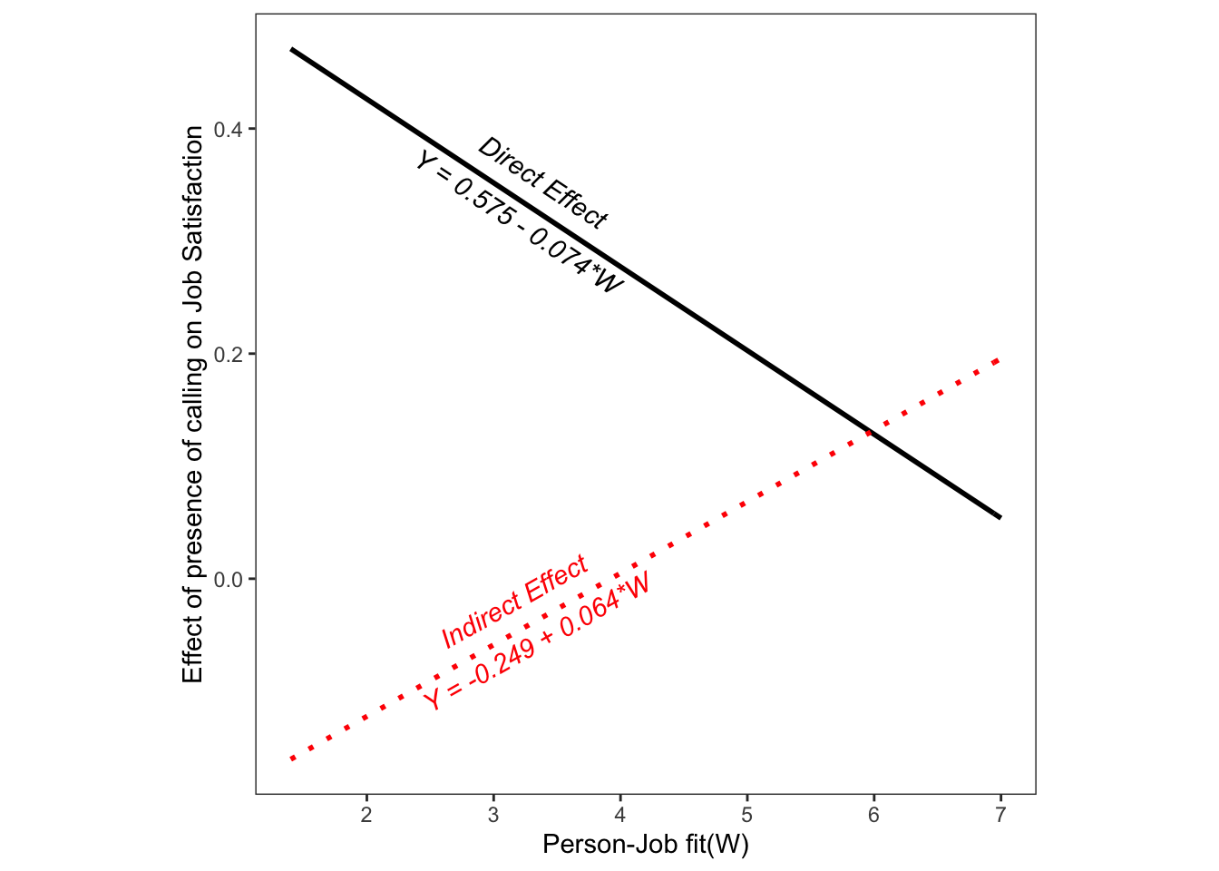
조절변수 Person-Job Fit에 따른 조건부 직접효과 및 간접효과는 다음과 같습니다.

modmedSummaryTable(semfit)

	Indirect Effect (a1+a3W)(b)
3.800	-0.008	(-0.134 to 0.140)	0.292	(0.004 to 0.564)
5.000	0.069	(-0.019 to 0.183)	0.203	(0.004 to 0.387)
5.800	0.119	(0.027 to 0.241)	0.143	(-0.024 to 0.312)
boot.ci.type = perc

조건부 직접효과와 간접효과를 다음과 같이 시작화 할 수도 있습니다.

conditionalEffectPlot(semfit, data=raw_data)+labs(x="Person-Job fit(W)", y="Effect of presence of calling on Job Satisfaction")

	Consequent
		Job_Satisfaction(Y)
Antecedent		Coef	SE	t	p
presence_of_calling(X)	c1	0.326	0.330	0.986	.326
Person_Job_fit(W)	c2	0.433	0.210	2.061	.041
presence_of_calling:Person_Job_fit(X:W)	c3	-0.011	0.062	-0.175	.862
Constant	iY	0.602	1.079	0.558	.578
Observations		151
R2		0.423
Adjusted R2		0.411
Residual SE		0.560 ( df = 147)
F statistic		F(3,147) = 35.907, p < .001