Chapter 5 Traditional Approach
Recap
I am looking to use a multiple linear regression model to predict house prices using a sample data set from the website Kaggle (2015). The data contains property sales prices for transactions between May 2014 and May 2015 in King County USA which includes Seattle.
I start by looking at any online literature on house price prediction. This “meta analysis” has two purposes:
- It helps select variables to include in the model
- It adds credibility to my findings if I incorporate and build on the empirical evidence of previous research studies
I then perform a formal model selection procedure. This involves:
- Variable selection
- Model fitting
- Diagnostics
- Selection between competing models
Having selected a final model, I then use the model to make predictions about property prices.
Meta Analysis
My data set only includes information on micro variables. These micro variables relate to the intrinsic features of a property and its immediate environment. By contrast, macro variables are excluded. These relate to the “external environment” of the property (see examples below).
By excluding macro variables, the parameter estimates of my model could be biased. For example, the data comes from the period from May 2014 to May 2015 when the external environment in the US was relatively stable. This means that the level of noise in the data could be artificially low and the explanatory power of micro variables overstated.
To mitigate this risk I have performed a quick online literature search and identified micro variables which previous research studies have found to be significant predictors of property price. I have included these variables as the starting point of the model selection process. This should lead as much overlap as possible between my model and previous studies and stops me relying 100% on a statistical model selection procedure which is vulnerable to bias.
Micro variable Examples
- Property location
- Building features
- Interior Layout
- Quality of fixture and fittings
Macro variable Examples
- National and local government policies
- the state of the mortgage market
- interest rates
- unemployment levels in the job market
- demographics
Results of online search
The table below shoes the micro-variables identified online, the reference article and the matching field in the database. Article 1 is (Galati, Teppa, and Alessie 2011), Article 2 is (Ezgi CANDAS and YOMRALIOGLU 2015), Website 1 is (RightMove 2017)
| Micro-variable | Reference | Data-Set Field |
|---|---|---|
| Year of Construction | Article 1 | Construction Year |
| Size of Living Room | Article 1 | Living Space |
| Presence of Garage | Article 1 | |
| Presence of Garden | Article 1 | |
| Type of House | Article 1 | Number of Floors |
| Large City vs not large | Article 1 | Seattle ZipCode |
| Degree of Urbanization | Article 1 | |
| Floor No | Article 2 | Floors |
| Heating System | Article 2 | Renovation Year |
| Earthquake Zone | Article 2 | |
| Rental Value | Article 2 | |
| Land Value | Article 2 | |
| Parcel Area | Article 2 | Total Area |
| Zoning | Article 2 | Zipcode |
| Proximity to Amenities | Website 1 | |
| Number of Bedrooms | Website 1 | Bedrooms |
| Number of Bathrooms | Website 1 | Bathrooms |
| Age of Building | Website 1 | |
| Condition of Interior | Website 1 | Condition/Grade |
Model Selection
Correlation Matrix
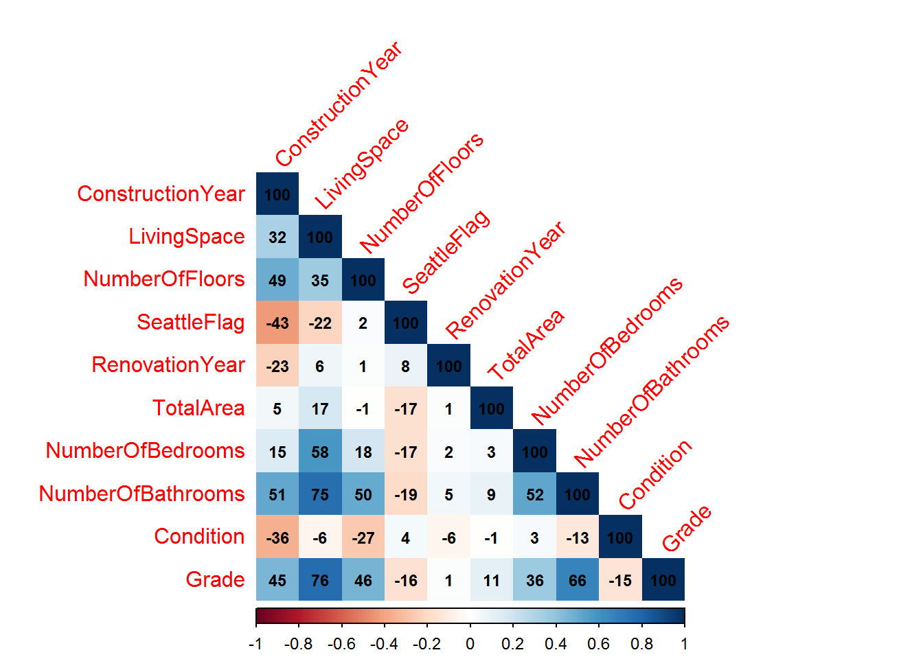
The correlation plot below shows that none of the data-set variables identified from the meta analysis are highly correlated (r>80%). This means they can all be included in the model without causing issues regarding multi-collinearity and non-convergence of the model fitting algorithm.

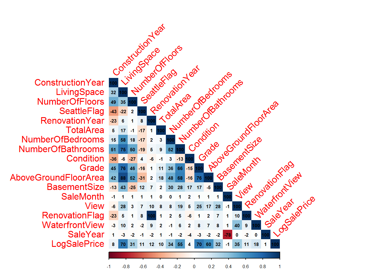
The full correlation plot for the data-set is shown below. The bottom row shows the correlations between the data-set variables and LogSalePrice. The top five correlated variables are LivingSpace, Grade,AboveGroundFloorArea, NumberOfBathrooms, View. All of which are positively correlated with LogSalePrice.

Model Fitting
Model 1 was fitted using only the variables identified in the meta-analysis. Models 2 to 5 were obtained using a step-wise AIC procedure to automatically select new models. Model 5 is where the procedure terminated.
| Model 1 | Model 2 | Model 3 | Model 4 | Model 5 | ||
|---|---|---|---|---|---|---|
| (Intercept) | 17.36*** | 17.14*** | 16.98*** | -65.15*** | -65.07*** | |
| (0.22) | (0.22) | (0.22) | (8.94) | (8.93) | ||
| ConstructionYear | -0.00*** | -0.00*** | -0.00*** | -0.00*** | -0.00*** | |
| (0.00) | (0.00) | (0.00) | (0.00) | (0.00) | ||
| LivingSpace | 0.00*** | 0.00*** | 0.00*** | 0.00*** | 0.00*** | |
| (0.00) | (0.00) | (0.00) | (0.00) | (0.00) | ||
| NumberOfFloors | 0.03*** | 0.03*** | 0.03*** | 0.03*** | 0.02*** | |
| (0.01) | (0.00) | (0.00) | (0.00) | (0.01) | ||
| SeattleFlag | 0.22*** | 0.22*** | 0.21*** | 0.21*** | 0.22*** | |
| (0.01) | (0.01) | (0.01) | (0.01) | (0.01) | ||
| RenovationYear | 0.00*** | 0.00*** | 0.00*** | 0.00*** | 0.00*** | |
| (0.00) | (0.00) | (0.00) | (0.00) | (0.00) | ||
| TotalArea | 0.00*** | 0.00*** | 0.00*** | 0.00*** | 0.00*** | |
| (0.00) | (0.00) | (0.00) | (0.00) | (0.00) | ||
| NumberOfBedrooms | -0.02*** | -0.02*** | -0.01*** | -0.01*** | -0.01*** | |
| (0.00) | (0.00) | (0.00) | (0.00) | (0.00) | ||
| NumberOfBathrooms | 0.07*** | 0.06*** | 0.06*** | 0.06*** | 0.06*** | |
| (0.00) | (0.00) | (0.00) | (0.00) | (0.00) | ||
| Condition | 0.06*** | 0.06*** | 0.06*** | 0.06*** | 0.06*** | |
| (0.00) | (0.00) | (0.00) | (0.00) | (0.00) | ||
| Grade | 0.22*** | 0.22*** | 0.21*** | 0.21*** | 0.21*** | |
| (0.00) | (0.00) | (0.00) | (0.00) | (0.00) | ||
| WaterfrontView | 0.52*** | 0.39*** | 0.39*** | 0.39*** | ||
| (0.02) | (0.03) | (0.03) | (0.03) | |||
| View | 0.04*** | 0.04*** | 0.04*** | |||
| (0.00) | (0.00) | (0.00) | ||||
| SaleYear | 0.04*** | 0.04*** | ||||
| (0.00) | (0.00) | |||||
| AboveGroundFloorArea | 0.00* | |||||
| (0.00) | ||||||
| R2 | 0.66 | 0.67 | 0.67 | 0.67 | 0.67 | |
| Adj. R2 | 0.66 | 0.67 | 0.67 | 0.67 | 0.67 | |
| Num. obs. | 21436 | 21436 | 21436 | 21436 | 21436 | |
| RMSE | 0.31 | 0.30 | 0.30 | 0.30 | 0.30 | |
| p < 0.001, p < 0.01, p < 0.05 | ||||||
The \(R^{2}\) value of Model 1 is 0.66. This seems relatively low with the regression fit only explaining circa 66% of the total variation about the mean.
The \(R^{2}\) value of Model 5 is 0.67. This also seems relatively low and only a small improvement on Fit 1. It is however statistically significant and we would reject the null hypothesis that the final model has no explanatory power in a formal test at the 0.1% level (see below).
| Model | DoF | RSS | DOF_Diff | SUmOfSq | FProb | |
|---|---|---|---|---|---|---|
| 1 | Fit1 | 21425.00 | 2018.00 | |||
| 2 | Fit5 | 21421.00 | 1952.00 | 4.00 | 65.65 | 0.00 |
I don’t think the improvement in fit in Model 5 is worth the extra four variable required and will use Model 1. For Model 1 it needs to be investigated further why the coefficients for NumberOfBedrooms and ConstructionYear have changed sign versus the values in the correlation matrix.
Diagnostics
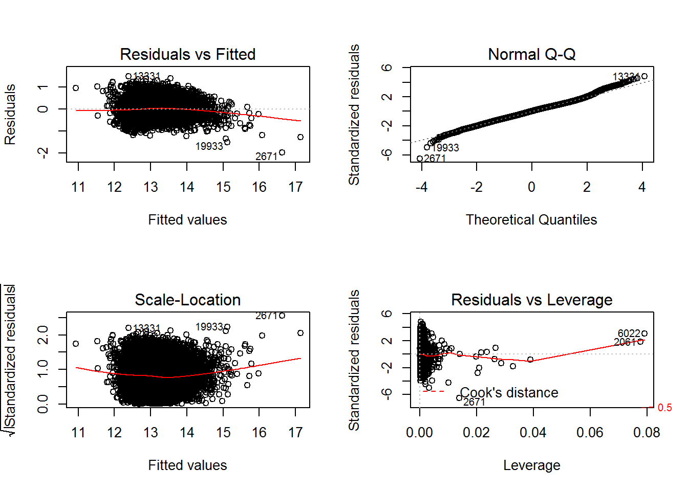
The chart below present visually key checks on whether the assumptions of the model are met. There is nothing to suggest that the residuals have a trend. The variability of the residuals does not change with fitted value and appears to follow a normal distribution. Two observations “6022” and “2061” have high leverage (influence on own fitted value) and high standardised residual (greater deviance from zero than expected). They do not have a Cook’s distance greater than 0.5 and hence do not have a material impact on fitted coefficient values.

Figure 5.1: Visual Checks on Model 1
References
Kaggle. 2015. “This Dataset Contains House Sale Prices for King County.” https://www.kaggle.com/harlfoxem/housesalesprediction.
Galati, Gabriele, Federica Teppa, and Rob JM Alessie. 2011. “Macro and Micro Drivers of House Price Dynamics: An Application to Dutch Data.”
Ezgi CANDAS, Seda BAGDATLI KALKAN, and Tahsin YOMRALIOGLU. 2015. “Determining the Factors Affecting Housing Prices.”
RightMove. 2017. “Positive and Negative Impacts on House Prices.” http://www.rightmove.co.uk/what-affects-house-prices.html.