Chapter 4 Geo Analysis
Visualising the data geospatially gives additional insights. In Figure 4.1, we see that our model from the previous section does not capture clusters of low value (dark blue) and high value properties (light purple).
## LogSalePrice ~ (ConstructionYear + LivingSpace + NumberOfFloors +
##     SeattleFlag + RenovationYear + TotalArea + NumberOfBedrooms +
##     NumberOfBathrooms + condition + grade) * FlatFlag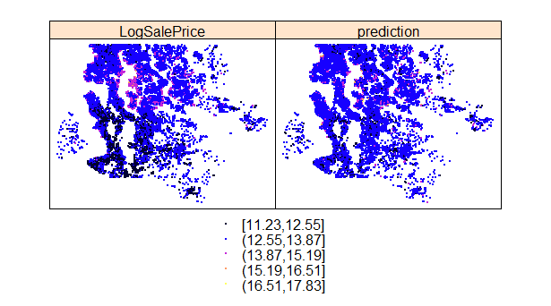
Figure 4.1: Fitting a model only on attributes of the property (eg. number of bedrooms) fails to predict all clusters of low value and high value properties.
If for each property in our data-set we add attributes of the neighbourhood, these explanatory variables allow us to model clusters more accurately. In Figure 4.2, the scales are slightly different but the cluster of high value properties (light purple) in the middle of the chart are predicted more accurately.
## LogSalePrice ~ condition + grade + SeattleFlag + RenovationYear +
##     TotalArea + NumberOfBedrooms + NumberOfBathrooms + LivingSpace +
##     NumberOfBedrooms + ConstructionYear + WaterfrontView + SeattleFlag +
##     Schools1000m + PoliceStation1000m + SupermarketGrocery750m +
##     DoctorDentist500m + BarNightclubMovie500m + NumberOfFloors +
##     ConstructionYear + WaterfrontView + SeattleFlag + Schools1000m +
##     PoliceStation1000m + SupermarketGrocery750m + Library750m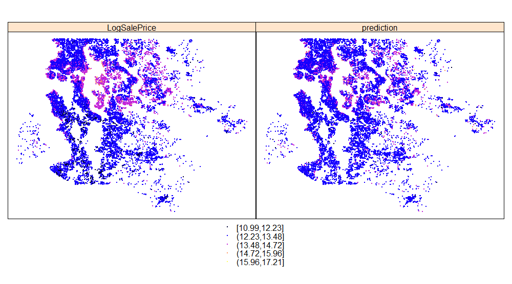
Figure 4.2: Fitting a model with property attributes & neighbourhood attributes as explanatory variables predicts some clusters better (eg. proximity of schools) .
The explanation for this is that we are failing to take account of how nice the neighbourhood is (eg. proximity to schools) when we only have attributes of a property as explanatory variables (eg. number of bedrooms).
Locational Data
In R, I used API calls to scrape data from the Google Maps and Zillow property websites. For each of the 21000 properties in the data-set, this involved passing the latitude and longitude co-ordinates to the website and receiving detailed neighbourhood data back.
The plots below show the data fields obtained in this way. The plots were created using the sp package in R. It is clear that some neighbourhood properties change significantly by location (eg. number of schools in 1000m). There are also variables which hardly change at all (eg. Number of Liquor Stores).
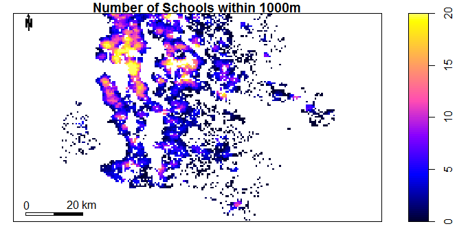
Figure 4.3: Number of Schools within 1000m by Location
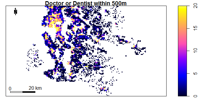
Figure 4.4: Number of Doctors or Dentists within 500m by Location
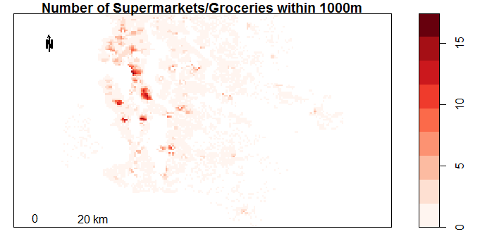
Figure 4.5: Number of Doctors or Dentists within 500m by Location
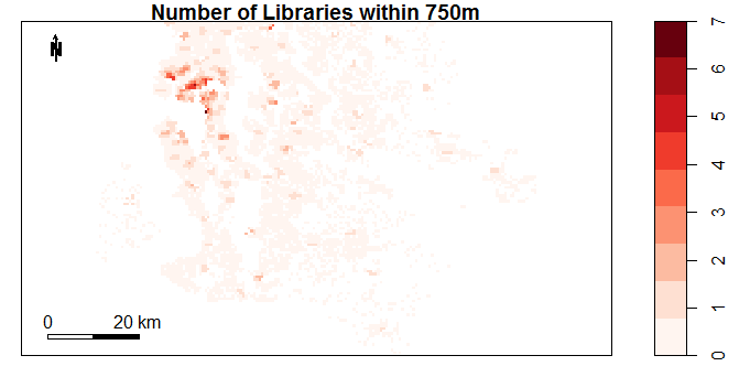
Figure 4.6: Number of Doctors or Dentists within 500m by Location
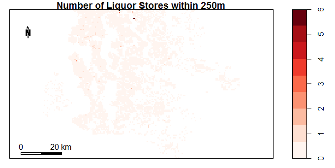
Figure 4.7: Number of Doctors or Dentists within 500m by Location
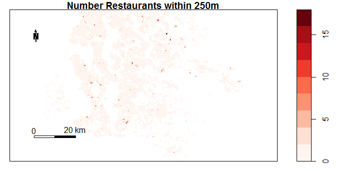
Figure 4.8: Number of Doctors or Dentists within 500m by Location
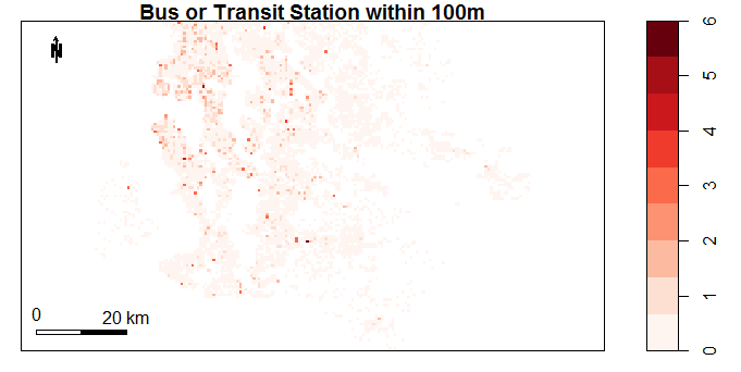
Figure 4.9: Number of Doctors or Dentists within 500m by Location
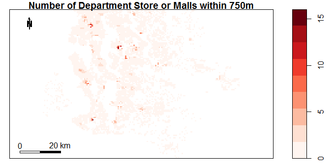
Figure 4.10: Number of Doctors or Dentists within 500m by Location
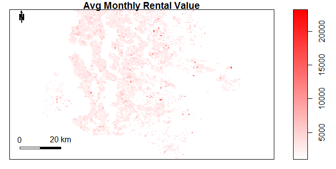
Figure 4.11: Number of Doctors or Dentists within 500m by Location
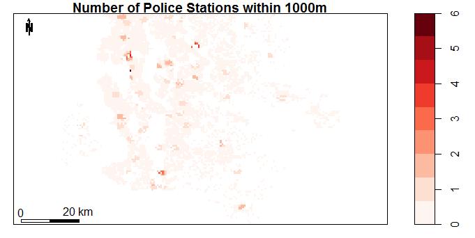
Figure 4.12: Number of Doctors or Dentists within 500m by Location
Other Data
It is suprising to find spatial patterns when we plot property specific variables (eg. Construction Year) by location. For example with Construction Year, the oldest properties are located in the north-west region and properties get progressively newer as we move east.
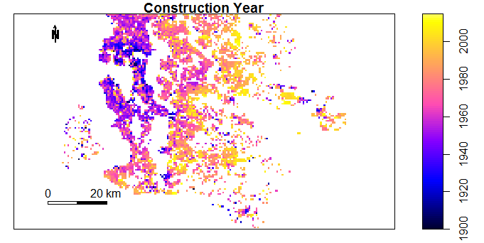
Figure 4.13: Number of Doctors or Dentists within 500m by Location
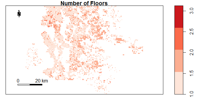
Figure 4.14: Number of Doctors or Dentists within 500m by Location
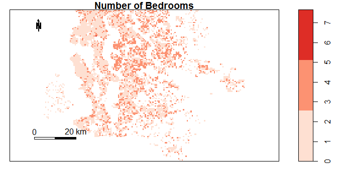
Figure 4.15: Number of Doctors or Dentists within 500m by Location
Statistics
For completeness, lets compare the model fitted with and without locational data.
| Model | DoF | RSS | DOF_Diff | SUmOfSq | FProb | |
|---|---|---|---|---|---|---|
| 1 | NonGeoModel | 21391.00 | 1997.00 | |||
| 2 | GeoModel | 21395.00 | 1823.00 | -4.00 | 173.45 |
| Model 1 | Model 2 | ||
|---|---|---|---|
| (Intercept) | 15.49*** | 15.76*** | |
| (0.22) | (0.39) | ||
| condition | 0.06*** | 0.09*** | |
| (0.00) | (0.01) | ||
| grade | 0.21*** | 0.21*** | |
| (0.00) | (0.00) | ||
| SeattleFlagYes | 0.14*** | 0.22*** | |
| (0.01) | (0.01) | ||
| RenovationYear | 0.00*** | 0.00*** | |
| (0.00) | (0.00) | ||
| TotalArea | 0.00*** | -0.00 | |
| (0.00) | (0.00) | ||
| NumberOfBedrooms | -0.02*** | -0.01 | |
| (0.00) | (0.00) | ||
| NumberOfBathrooms | 0.05*** | 0.03*** | |
| (0.00) | (0.01) | ||
| LivingSpace | 0.00*** | 0.00*** | |
| (0.00) | (0.00) | ||
| ConstructionYear | -0.00*** | -0.00*** | |
| (0.00) | (0.00) | ||
| WaterfrontView | 0.59*** | ||
| (0.02) | |||
| Schools1000m | 0.02*** | ||
| (0.00) | |||
| PoliceStation1000m | -0.02*** | ||
| (0.00) | |||
| SupermarketGrocery750m | -0.03*** | ||
| (0.00) | |||
| DoctorDentist500m | 0.00*** | ||
| (0.00) | |||
| BarNightclubMovie500m | 0.01*** | ||
| (0.00) | |||
| NumberOfFloors | 0.00 | 0.04** | |
| (0.00) | (0.01) | ||
| Library750m | 0.03*** | ||
| (0.00) | |||
| FlatFlag1 | 3.13*** | ||
| (0.52) | |||
| ConstructionYear:FlatFlag1 | -0.00*** | ||
| (0.00) | |||
| LivingSpace:FlatFlag1 | 0.00 | ||
| (0.00) | |||
| NumberOfFloors:FlatFlag1 | -0.01 | ||
| (0.02) | |||
| SeattleFlagYes:FlatFlag1 | -0.03* | ||
| (0.01) | |||
| RenovationYear:FlatFlag1 | -0.00 | ||
| (0.00) | |||
| TotalArea:FlatFlag1 | 0.00*** | ||
| (0.00) | |||
| NumberOfBedrooms:FlatFlag1 | -0.02*** | ||
| (0.01) | |||
| NumberOfBathrooms:FlatFlag1 | 0.05*** | ||
| (0.01) | |||
| condition:FlatFlag1 | -0.04*** | ||
| (0.01) | |||
| grade:FlatFlag1 | 0.03*** | ||
| (0.01) | |||
| R2 | 0.69 | 0.66 | |
| Adj. R2 | 0.69 | 0.66 | |
| Num. obs. | 21413 | 21413 | |
| RMSE | 0.29 | 0.31 | |
| p < 0.001, p < 0.01, p < 0.05 | |||