7 Discover dissatisfaction drivers with Multiple Linear Regression
There are many applications of regression in human-centered research. Today, I’ll focus on something called a “drivers analysis”. It’s a technique that identifies which variables most significantly “drive”, or “impact”, an overall variable. This shows a company where to best concentrate its efforts for improving metrics like overall satisfaction with an product or Net Promoter Score (NPS).
Regression models take an outcome variable and a set of predictor variables as input. The regression model tells us the relationship between the predictor variables and the outcome variable, specifically how the predictor variables “impact” the outcome variable (if at all). Visually, we can think of linear regressions as lines or planes that “best fit” our data. And these lines and planes can be represented as an equation as well.
\(Y\) = outcome variable
\(x_{n}\) = predictor variable n
\(beta_{n}\) = coefficient of predictor variable n
\(beta_{0}\) = intercept/constant
One of the most important things for us is the sign and the magnitude of the coefficient for each of the predictor variables. Again, this tells us how each predictor variable “impacts” the outcome variable.
7.1 Introduction
Let’s back up a bit and talk about how to select outcome and predictor variables. Put simply, an outcome variable is a metric that is important to your company and something your company wants to improve or influence. This could be something like overall satisfaction with a product or service. It could also be a metric your company tracks such as Customer Satisfaction Score (CSAT) or Net Promoter Score (NPS).
You also must collect relevant predictor variables in the survey. Use your subject-matter expertise and think of which variables might be related to or have an influence on the outcome variable of interest.
For example, take the case of a simple app with 4 major features. Our outcome variable is overall satisfaction with the app. And our predictor variables will be individual satisfaction ratings for each of the 4 features. Let’s also throw in a customer experience score as a final predictor. In total we have 5 predictor variables and we will regress them on “overall app satisfaction”.
Make sure to write out your hypotheses before fitting the model. This helps clarify your thinking and rationale for conducting a regression analysis in the first place.
\(H_{0}: \beta_{1} = \beta_{2} = \beta_{3} = \beta_{4} = \beta_{5} = 0\)
\(H_{1}\): At least one \(\beta\) is non-zero
A note on model interpretability: Most resources warn against increasing model complexity by adding many predictor variables. The best models are parsimonious and easy to explain in simple terms.
7.2 Analysis
It is helpful to get your variables all in one place. Create a data frame that contains your predictor variables and the outcome variable. In this case, the first 5 columns are our predictor variables and the last is our outcome variable (i.e. overall app satisfaction). Each of the variables in our data set are likert scale satisfaction ratings from 0 to 100.
##   CX_score featureA featureB featureC featureD overall
## 1       70       85       74       61       56      79
## 2       66       80       63       55       49      65
## 3       67       74       59       49       39      58
## 4       63       79       62       52       38      61
## 5       71       82       69       54       47      48
## 6       75       77       64       49       39      62
7.2.1 Linear Model Assumptions
Like all parametric techniques, regression models come with assumptions about the data.
- Each variable follows a normal distribution
- Linear relationship between the predictor variables and the dependent variable. Any predictor variables that do not meet this criterion may need to be transformed (e.g. log).
We can check both of these assumptions by looking at histograms and scatterplots of the predictors versus the outcome.
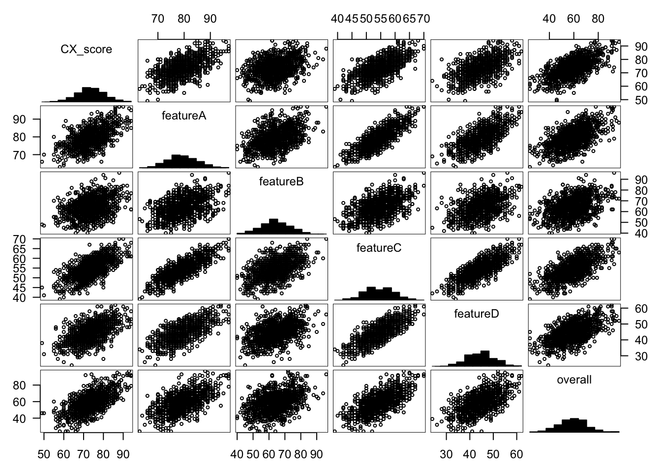
Indeed, all variables are normally distributed. Looking at the sixth column, we see eliptical scatterplot patterns, which indicate linear relationships between the predictor variables and the outcome variable. They are also positively correlated with one another which makes intuitive sense: as feature satisfaction levels increase, we expect overall app satisfaction to increase as well.
- Finally, multicollinearity can present a problem in linear regressions. When predictor variables are highly correlated with each other it makes coefficient estimation difficult. Let’s take the extreme example that feature A and feature B satisfaction ratings are perfectly colinear with each other (+1.0). These variables appear identical to the model so the model will not be able to decide which is the more important of the two for explaining the variance in the outcome variable.
The matrix below shows all correlations between the predictors. We’re hoping for correlation values closer to zero. Correlations of magnitude greater than .8 may cause concern. Issues of multicollinearity can more accurately be diagnosed by calculating Variable Inflation Factor (VIF) for the predictors; however, we must first fit the model before calculating VIF, so the correlation matrix is a good initial check for right now.
##          CX_score featureA featureB featureC featureD
## CX_score     1.00     0.59     0.35     0.66     0.56
## featureA     0.59     1.00     0.48     0.82     0.68
## featureB     0.35     0.48     1.00     0.52     0.44
## featureC     0.66     0.82     0.52     1.00     0.78
## featureD 0.56 0.68 0.44 0.78 1.00- Finally, in order to compare their relative importance, predictor variables must be on the same scale as one another. For example, if one of your predictor variables is on a 1-7 scale and the others are on a 0-100 scale, the predictors must be standardized.
7.3 Fit Model
Linear models can be fit with one line in R. “overall” denotes our outcome variable and the “.” selects all other variables in the data frame as predictor variables for the model.
7.3.1 Check Model Fit
Now that we have a model we will want to check how well it fits our data and that it satisfies several other assumptions.
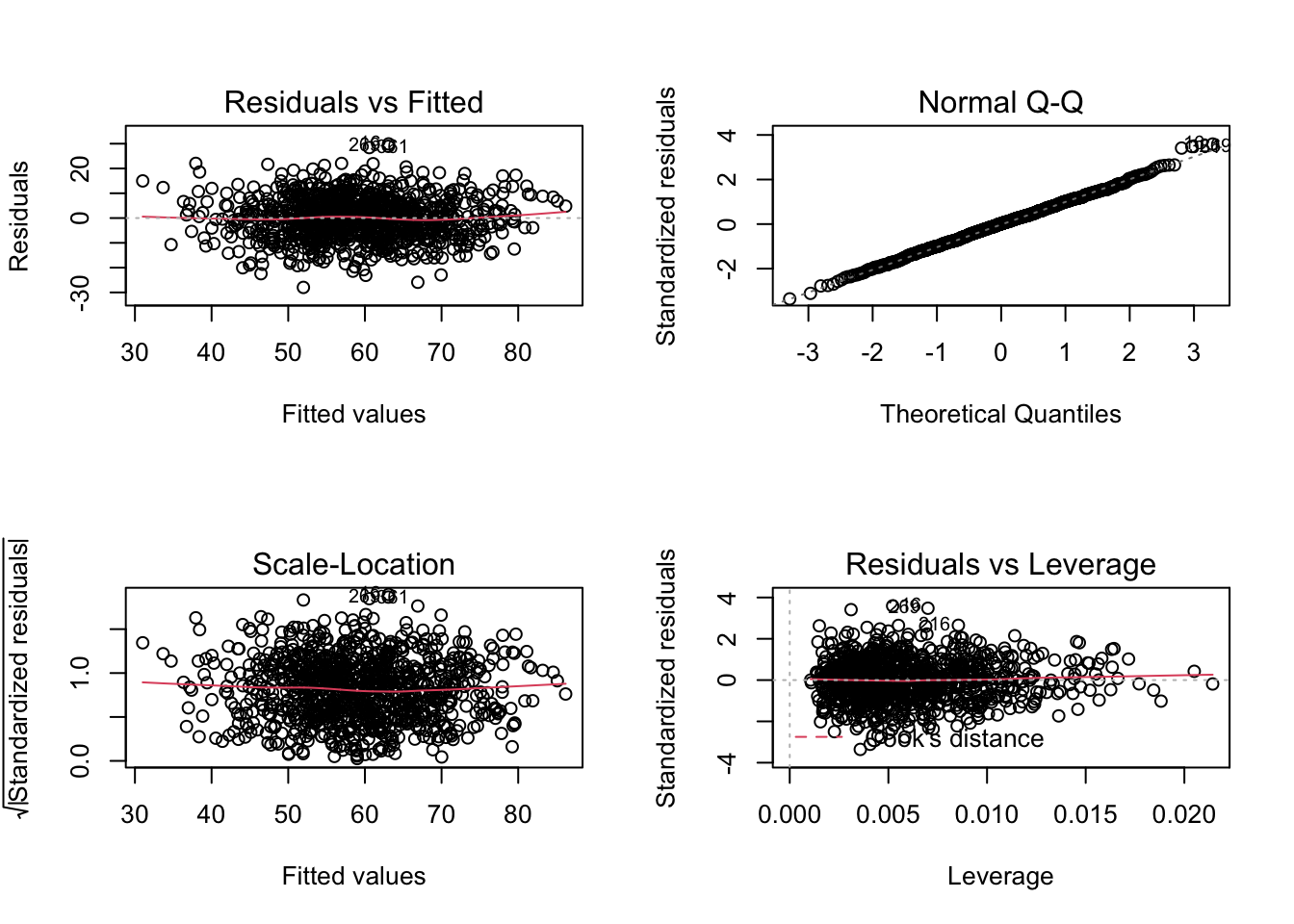
- Residuals should follow a normal distribution If they do not, this is usually because of a non-linear relationship between a predictor and the outcome. We already checked for this, so we should be good. See quadrant I below.
- No pattern in the residuals across the model’s predicted (or “fitted”) values. If the residuals aren’t evenly distributed then it violates the assumption of homoscedasticity. See quadrant II and III below.
- Outliers, or “abnormal” data points, with high residuals can disproportionately skew our overall model The influence that a data point has on the model is described with a metric called Cook’s Distance. Some outliers may be caused by data entry errors on the researcher or respondents’ behalf. The model should be re-fit after removing these problematic outliers. See quadrant IV below.
- Let’s check for multicollinearity issues in our model with Variable Inflation Factors (VIF) VIF scores above 5 or 10 are considered problematic and likely necessitate the removal of highly correlated variables. VIF scores are low in this case.
## CX_score featureA featureB featureC featureD
## 1.795359 3.212558 1.388939 4.817432 2.609611
7.3.2 Interpreting Model Results
Now lets actually interpret the model’s output.
##
## Call:
## lm(formula = overall ~ ., data = dat)
##
## Residuals:
##      Min       1Q   Median       3Q      Max
## -27.9772  -5.8887   0.1351   5.5201  29.9088
##
## Coefficients:
##              Estimate Std. Error t value Pr(>|t|)
## (Intercept) -45.35646    3.86624 -11.731  < 2e-16 ***
## CX_score      0.62012    0.05002  12.397  < 2e-16 ***
## featureA      0.16912    0.08230   2.055  0.04014 *
## featureB      0.06345    0.03466   1.831  0.06744 .
## featureC      0.57214    0.11536   4.959 8.31e-07 ***
## featureD      0.22867    0.07105   3.218  0.00133 **
## ---
## Signif. codes:  0 '***' 0.001 '**' 0.01 '*' 0.05 '.' 0.1 ' ' 1
##
## Residual standard error: 8.348 on 994 degrees of freedom
## Multiple R-squared:  0.5238, Adjusted R-squared:  0.5214
## F-statistic: 218.7 on 5 and 994 DF,  p-value: < 2.2e-16
First of all, the F-statistic at the bottom tests our original hypothesis:
\(H_{1}\): At least one \(\beta\) is non-zero
With such a small p-value, we reject the null hypothesis and can say with certainty that at least one of the predictors significantly impacts overall app satisfaction. In other words, at least one of the coefficients is not equal to zero. The model gives us the coefficient (i.e. “Estimate”) for each predictor variable and runs a t-test to check whether or not each coefficient is significantly greater than or less than 0.
We can quickly visualize sign, magnitude and confidence intervals of the coefficients with the following plot.
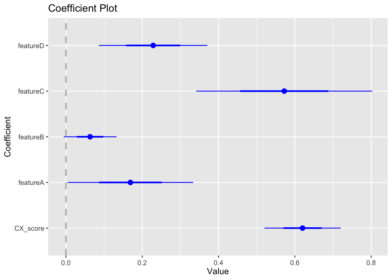
Things are looking good, here are my key take-aways:
All predictors are statistically significant at the 95% confidence interval, except for “featureB”
All coefficients have a positive sign, meaning that as the value of the predictors increase, we would expect an increase in “overall app satisfaction”. This makes intuitive sense and is in-line with our correlation matrix above.
“CX_score” and “featureC” have the largest coefficients by far
The 5 predictors explain 52% of the variance in “overall app satisfaction” for this data set (as per adjusted R-squared)
7.3.3 Adjusted R-squared
Adjusted R-squared is an important metric as it tells us how well our model fits the data. As errors between the predicted and actual values increase, R-squared decreases. Another way of thinking about it is the amount of variation in the outcome variable explained by the model. It’s a score from 0 to 1, where 1 indicates that the model explains 100% of the variation in the outcome variable. STEM fields that model systems with stable and fundamental laws tend to have higher R-squared values compared to Behavioral and Human Sciences, which typically have more unexplained variance and R-squared values that rarely exceed .50.
In our case, the 5 predictors explain 52% of the variance in “overall app satisfaction”. It’s easy to think of other predictors that might explain higher or lower overall app satisfaction. For instance, I’d be interested in fitting a model with “age” and “gender” also included. Lower R-squared values are okay for our purposes since the model still explains the relative importance of predictors.
7.4 Variable Selection
We only used 5 predictors in this case, but a typical drivers analysis might include dozens of satisfaction ratings. Adding predictors will only increase the adjusted R-squared, generating a seemingly better model; however, estimates of the coefficients will become less precise and could lead to incorrect interpretations of relationships in the data (Chapman and Feit 2019).
This problem of “over-fitting” can be mitigated by selecting the most important variables to include in the final model. Perhaps the most popular way of handling this is with a method known as step-wise regression. In one type of step-wise regression, backward selection, a model is fit with all predictors of interest. Variables are then removed one-by-one based on a criterion like largest p-value until all are under .05, or maximizing adjusted R-squared, or optimizing other metrics like AIC/BIC.
“Over-fitting” is especially a problem when using the model for prediction. It is less of an issue for explanatory model with only 5 predictors. In any case, models with many predictor variables should consider step-wise regression.
7.5 Final Analysis & Recommendations
Everything is in order, now we need to present the results to our product development team so that they can prioritize improvements. Our regression model tells us the relative importance of the predictors (\(\beta\)’s). We also know the average satisfaction for each of the predictors. Let’s combine this information into a final driver’s analysis deliverable and discuss implications.
coef <- as.numeric(signif(m1$coefficients[2:length(m1$coefficients)],2))
var <- names(m1$coefficients[2:length(m1$coefficients)])
var.sat <- signif(c(mean(dat[,"CX_score"]), mean(dat[,"featureA"]),
             mean(dat[,"featureB"]), mean(dat[,"featureC"]),
             mean(dat[,"featureD"])), 2)

df <- data.frame(coef, var.sat, row.names = var)

ggplot(df, aes(x=var.sat, y=coef)) + geom_point() +
        theme(legend.title=element_blank()) +
        labs(title="Product Development Decision Matrix",
             x="Satisfaction", y= "Coefficients") +
        geom_hline(yintercept = (((range(coef)[[2]] - range(coef)[[1]])/2)
                           + range(coef)[[1]])) +
        geom_vline(xintercept = (((range(var.sat)[[2]] - range(var.sat)[[1]])/2)
                           + range(var.sat)[[1]])) +
        geom_label(aes(var.sat, coef, label=row.names(df)), nudge_y = .05)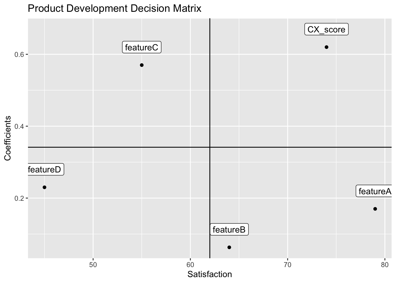
Average predictor satisfaction is on the x-axis and predictor coefficients are on the y-axis (Sauro 2016).
Quadrant I: High satisfaction + High importance
Leverage and expand the Customer Experience score
Quadrant II: Low satisfaction + High importance
Prioritize improvements on featureC, because improving its satisfaction has a high impact on overall app satisfaction
Quadrant III: Low satisfaction + Low importance
Feature D is low priority
Quadrant IV: High satisfaction + Low importance
Maintain the high satisfaction of Feature A and Feature B with minimal effort
Bibliography
Chapman, C, and E Feit. 2019. R for Marketing Research and Analytics. New York, NY: Springer Berlin Heidelberg.
Sauro, Jeff. 2016. “Measuringu: 10 Things to Know About a Key Driver Analysis.” MeasuringU. https://measuringu.com/key-drivers/.