6 Measure UX and track product improvement with Usability Testing
As user researchers or product managers, we start with a need to understand the attitudes and product usage of a population of users to guide product design; however, it’s almost never feasible to study every user in the population - just think of popular social media platforms with hundreds of millions, even billions, of users. Fortunately, the field of inferential statistics gives a framework for sampling users from a population, studying this subset of users, and making inferences about the population based on measurements from the sample.
Taking measurements on a subset of the population is sub-optimal because it is an approximation of the population, and thus, introduces sampling error (Särndal et al. 2003). With inferential statistics we can describe our confidence in how sample measurements relate to the population values with something called confidence intervals. A point estimate and confidence interval might be reported to stakeholders like the following: “the SUS score for new users of MetaMask wallet is 52 with a confidence interval of 46 to 59 at the 95% confidence level”. Smaller confidence intervals mean that our sample estimates are more precise. Obtaining a larger sample size is the main way to make confidence intervals smaller - but more on this later.
Hypothesis testing is another function of inferential statistics. For example, we may measure differences between two different user groups in a sample, like MetaMask users versus Coinbase users. With hypothesis testing, we can decide if there is enough evidence to say that these are real differences that also exist in the population, or if these differences are just attributed to noise in our sample (Särndal et al. 2003).
6.1 Introduction
In this project, our goal is to compare the usability of three crypto wallets (MetaMask, Argent, and Coinbase). The populations of interest are new users of these three platforms; therefore, we sample these user populations and apply inferential techniques like calculating confidence intervals around all point estimates and testing for statistically significant differences between the three groups. Again, this allows us to make claims about the populations of interest with statistical confidence, based on the sample measurements we collect during the usability tests.
There are many types of usability tests. We are interested in a comparative, as well as a summative usability test. “Comparative” in that three different products are included in the study, and we want to end with an understanding of their relative usability to one another. “Summative” in that we are measuring the performance of mature, high-fidelity products and prioritize quantitative evaluation on pre-defined metrics (like task completion) as opposed to issue discovery (Joyce 2019). “Measuring the User Experience” is a great resource when designing these summative usability tests - it mentions three different question types that might be included in such a study (Tullis and Albert 2013).
- Task performance metrics (Completion rate, Time on task, Errors, Efficiency, Learnability)
- Post-Task Ratings (Ease-of-use, Expectations, ASQ)
- Post-Session Questionnaire (System Usability Score)
Generally, designing a summative usability test begins by specifying the tasks we wish to evaluate. These may be the most common or critical tasks for users, thus we want to ensure great performance on each. These tasks can also be related to areas that were changed in the previous design sprint, and we want to validate these newly improved areas of the product.
6.2 Data Collection
For our purposes, each crypto wallet is evaluated on 5 tasks. We take two point measurements for each task: whether or not the user successfully completed the task (pass/fail) and, if the user did complete the task, the time it took for him or her to complete it. Finally, at the end, we give the respondent an SUS questionnaire to assess the overall usability of the wallets. You can find out more about this questionnaire and scoring the SUS here.
This brings us to the question of sample size. Usability testing is resource intensive, especially when it’s in-person; the more sample we have, the smaller our confidence intervals, and the smaller differences we can detect on usability measurements between the wallets. Thus, we must think about sample size carefully, and balance precision with pragmatism. In Chapter 6 of “Quantifying the User Experience”, Sauro provides a detailed, mathematically-based approach for estimating the sample size needed, based on several parameters like critical difference, confidence level, and estimated variability (Sauro and Lewis 2016). We want to be able to detect 20%+ differences between wallets at the 85% confidence level, which suggests that we need a sample size of 10n. Our sample isn’t too costly so we add 5, for a sample size of 15n.
There are two-types of study designs: between-subject and within-subject (Budiu 2018). Within-subject designs test all three products with the 15 users. On the other hand, between-subject designs, test only one wallet with each user. Both have their pros and cons. Within-subject designs can bias users because they are shown multiple concepts, which can affect their performance on subsequent wallets (due to task learning). We can randomize the order wallets are tested with users, which should mitigate this ordering bias; however, the concern still remains. Also, within-subject studies are longer and may fatigue the user as the test proceeds.
Between-subject designs do not suffer from this ordering bias, but require greater sample because only one wallet is tested with each user. We proceed with a between-subject design and multiply our total sample by three to maintain the precision we calculated in the paragraph above. Thus, our final sample size is 45n, with 15n wallet sub-groups.
Finally, our sample must be representative of the population - this is a fundamental assumption in inferential statistics. Imagine that our population of users has an average age of 25. There is a significant skew if the average age in our sample is 50 - it isn’t a good representation of the population. Crypto wallet usability likely differs by a significant degree between the population and this sample.
Proper representation is achieved by randomly sampling users from the population - hence the oft-cited term “random representative sample”. This is great in theory, but virtually impossible in practice. There are many sampling biases outside of the researcher’s control, like the fact that some users from the population are less likely to participate in the survey (e.g. males). Just be aware of these potential issues and seek the counsel of recruiting services who have experience troubleshooting these problems.
The usability test protocol is specified below. Again, for each task we collect two performance measurements, completion rate and time on task. And, an SUS questionnaire is given at the end of the study.
key <- list("Task 1" = "Setup app",
            "Task 2" = "Deposit crypto in wallet from CEX",
            "Task 3" = "Send crypto to friend",
            "Task 4" = "Connect hardware wallet",
            "Task 5" = "Connect AAVE DApp",
            "Post-Session Questionnaire" = "System Usability Score (SUS)")
print(key)
## $`Task 1`
## [1] "Setup app"
##
## $`Task 2`
## [1] "Deposit crypto in wallet from CEX"
##
## $`Task 3`
## [1] "Send crypto to friend"
##
## $`Task 4`
## [1] "Connect hardware wallet"
##
## $`Task 5`
## [1] "Connect AAVE DApp"
##
## $`Post-Session Questionnaire`
## [1] "System Usability Score (SUS)"
6.3 Analysis
The “Completion” variables are binary and coded as either Pass (1) or Fail (0). These variables will be described as proportions (e.g. only 60% of new MetaMask users completed Task 1). On the other hand, the “Time” variables are continuous and a measure of the seconds that elapsed during the completion of a task. We use mean to describe these variables (e.g. on average it takes 352 seconds for new MetaMask users to complete Task 1). Note that if the user did not complete a task then his/her time measurement was discarded for that task. These cases are coded as “NA”, and can be seen below.
##    T1_Completion T1_Time T2_Completion T2_Time T3_Completion T3_Time
## 1           Pass     378          Pass     263          Pass       5
## 2           Pass     397          Pass     235          Fail      NA
## 3           Fail      NA          Pass     249          Fail      NA
## 16          Pass     211          Pass     232          Fail      NA
## 17          Pass     141          Pass     227          Pass     107
## 18          Pass     205          Fail      NA          Pass      61
## 30          Pass     207          Pass     232          Pass      78
## 31          Fail      NA          Pass      44          Pass      87
## 32          Pass     174          Pass      71          Pass     118
##    T4_Completion T4_Time T5_Completion T5_Time SUS     User
## 1           Pass     159          Pass     109  39 MetaMask
## 2           Fail      NA          Fail      NA  52 MetaMask
## 3           Pass     284          Pass     118  66 MetaMask
## 16          Pass     268          Pass     284  52   Argent
## 17          Pass     457          Fail      NA  80   Argent
## 18          Fail      NA          Fail      NA  84   Argent
## 30          Fail      NA          Fail      NA  60   Argent
## 31          Fail      NA          Pass     302  98 Coinbase
## 32          Fail      NA          Pass     229  72 Coinbase
Let’s now calculate completion rate and mean time for the three crpyto wallets on Task 1.
#Task 1
prop <- prop.table(table(dat$T1_Completion,dat$User), margin  = 2)[2,]
prop <- data.frame(names(prop), prop)
names(prop)[1] <- "product"
prop[,2] <- round(prop[,2], 2)

m <- aggregate(dat$T1_Time ~ dat$User, FUN = mean, na.rm = TRUE)
names(m)[1] <- "product"
m[,2] <- round(m[,2], 0)

T1 <- merge(x = prop, y = m)
names(T1) <- c("Product","% Complete", "Time")

print(T1)
## Product % Complete Time
## 1 Argent 0.93 188
## 2 Coinbase 0.87 124
## 3 MetaMask 0.60 354These are the sample estimates for Task 1, but how confident are we in their estimation of the true population values? For this we will calculate confidence intervals. Also, we see differences between the three wallets, but do these differences really exist in the population? For this we use hypothesis testing, in search of statistically significant differences.
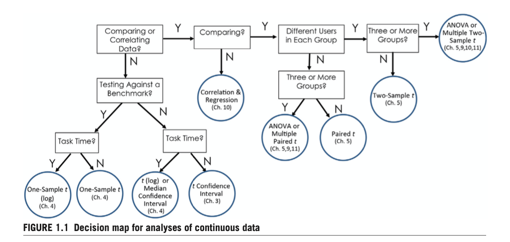
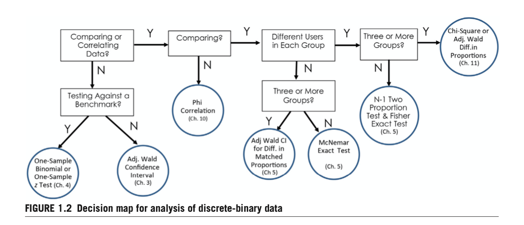
The analysis is broken into two sections (proportions and continuous) because different variable types require different statistical tests. In his comprehensive book “Quantifying the User Experience”, Jeff Sauro provides decision trees for deciding which statistical tests to use (Sauro and Lewis 2016). We base our analyses on his recommendations.
6.3.1 Frequency Data & Fisher Exact Tests
In this section we analyze the discrete-binary “Completion” variables. We can count the number of times that users pass and fail at a specific task, and see this for each wallet. These are called contingency tables. With three wallets and two outcomes (pass/fail), we will generate 3x2 contingency tables.
# Count number of passes for each task and each wallet
MM1 <- sum(dat[dat[,"User"] == "MetaMask","T1_Completion"] == "Pass")
MM2 <- sum(dat[dat[,"User"] == "MetaMask","T2_Completion"] == "Pass")
MM3 <- sum(dat[dat[,"User"] == "MetaMask","T3_Completion"] == "Pass")
MM4 <- sum(dat[dat[,"User"] == "MetaMask","T4_Completion"] == "Pass")
MM5 <- sum(dat[dat[,"User"] == "MetaMask","T5_Completion"] == "Pass")

AG1 <- sum(dat[dat[,"User"] == "Argent","T1_Completion"] == "Pass")
AG2 <- sum(dat[dat[,"User"] == "Argent","T2_Completion"] == "Pass")
AG3 <- sum(dat[dat[,"User"] == "Argent","T3_Completion"] == "Pass")
AG4 <- sum(dat[dat[,"User"] == "Argent","T4_Completion"] == "Pass")
AG5 <- sum(dat[dat[,"User"] == "Argent","T5_Completion"] == "Pass")

CB1 <- sum(dat[dat[,"User"] == "Coinbase","T1_Completion"] == "Pass")
CB2 <- sum(dat[dat[,"User"] == "Coinbase","T2_Completion"] == "Pass")
CB3 <- sum(dat[dat[,"User"] == "Coinbase","T3_Completion"] == "Pass")
CB4 <- sum(dat[dat[,"User"] == "Coinbase","T4_Completion"] == "Pass")
CB5 <- sum(dat[dat[,"User"] == "Coinbase","T5_Completion"] == "Pass")

# Use counts to create 3x2 contingency tables for Exact Fisher Tests
t1 <- matrix(c(MM1, AG1, CB1,15-MM1, 15-AG1, 15-CB1),
             nrow = 3,
             dimnames = list(Product = c("MetaMask","Argent", "Coinbase"),
                             Completion = c("Pass", "Fail")))

t2 <- matrix(c(MM2, AG2, CB2, 15-MM2, 15-AG2, 15-CB2),
       nrow = 3,
             dimnames = list(Product = c("MetaMask","Argent", "Coinbase"),
                             Completion = c("Pass", "Fail")))

t3 <- matrix(c(MM3, AG3, CB3, 15-MM3, 15-AG3, 15-CB3),
             nrow= 3,
             dimnames = list(Product = c("MetaMask","Argent", "Coinbase"),
                             Completion = c("Pass", "Fail")))


t4 <- matrix(c(MM4, AG4, CB4, 15-MM4, 15-AG4, 15-CB4),
             nrow= 3,
             dimnames = list(Product = c("MetaMask","Argent", "Coinbase"),
                             Completion = c("Pass", "Fail")))

t5 <- matrix(c(MM5, AG5, CB5, 15-MM5, 15-AG5, 15-CB5),
             nrow= 3,
             dimnames = list(Product = c("MetaMask","Argent", "Coinbase"),
                             Completion = c("Pass", "Fail")))
print(t5)
## Completion
## Product Pass Fail
## MetaMask 12 3
## Argent 6 9
## Coinbase 12 3The 3x2 contingency table for Task 5 is printed as an example above. It shows that 12 MetaMask users and 12 Coinbase users passed Task 5, whereas, only 6 Argent users passed Task 5. Now we want to test if any of these frequencies are significantly different than we’d expect from chance. In other words, we test whether or not the wallet variable is independent of the completion rate for Task 5. Most commonly, a chi-squared test is used when testing 3 or more frequencies at once; however, the Fisher Exact Test is recommended with small sample sizes and when cell sizes are less than 5n (Sauro and Lewis 2016). Thus, we proceed with the Fisher Exact Test and the following hypotheses for each task:
\(H_{1}\): At least one proportion is different than expected
##
##  Fisher's Exact Test for Count Data
##
## data:  t1
## p-value = 0.1067
## alternative hypothesis: two.sided##
## Fisher's Exact Test for Count Data
##
## data: t2
## p-value = 1
## alternative hypothesis: two.sided##
## Fisher's Exact Test for Count Data
##
## data: t3
## p-value = 0.166
## alternative hypothesis: two.sided##
## Fisher's Exact Test for Count Data
##
## data: t4
## p-value = 0.004543
## alternative hypothesis: two.sided##
## Fisher's Exact Test for Count Data
##
## data: t5
## p-value = 0.04445
## alternative hypothesis: two.sidedP-values are equal to 1 - (confidence level). So if we set the confidence level to 95% (as is customary), then we reject the null hypothesis on Tasks 4 and 5. This means that at least one of the frequencies significantly differs from expectation on Tasks 4 and 5, but we don’t know which one. Let’s visualize the proportions on Tasks 4 and 5 and then follow-up with further stat-testing to determine which wallets’ completion rates differ from expectation.
First, let’s calculate the confidence intervals using something called an adjusted-Wald test, so that we can add the confidence intervals to our visual. The normal Wald test doesn’t do well with small samples sizes of 100 or less (Sauro and Lewis 2016).
# Task 4 Completion CI's
MM <- addz2ci(x = t4[1,1], n = 15, conf.level = .85)
AG <- addz2ci(x = t4[2,1], n = 15, conf.level = .85)
CB <- addz2ci(x = t4[3,1], n = 15, conf.level = .85)

plot.dat <- data.frame(Product = c("MetaMask", "Argent", "Coinbase"),
                       Estimate = round(c(MM$estimate, AG$estimate, CB$estimate),2),
                       Lower = round(c(MM$conf.int[1], AG$conf.int[1], CB$conf.int[1]),2),
                       Upper = round(c(MM$conf.int[2], AG$conf.int[2], CB$conf.int[2]),2))

plot.dat
## Product Estimate Lower Upper
## 1 MetaMask 0.82 0.69 0.96
## 2 Argent 0.59 0.42 0.76
## 3 Coinbase 0.29 0.14 0.45Now we have point estimates, and lower and upper bounds of the confidence interval for task completion on Task 4. Confidence intervals can be tricky to interpret, they literally mean: “the range of possible estimates that we would expect to see 95% of the time if we repeatedly estimate a statistic using random samples from a population” (Chapman and Feit 2019). In other words, it’s the best guess of possible values in randomly drawn samples. Notice that the confidence intervals are relatively large ranges (~40% range) in our case - this is what we get when using small sample sizes of 15n. We can make confidence intervals smaller by decreasing our confidence level, or increasing sample.
Also note that the point estimates shown above are slightly different than if we were to calculate completion rates from the raw data, because the adjusted-Wald adds two successes and two failures for better accuracy at smaller samples sizes (Sauro and Lewis 2016). We end up reporting raw point estimates to stakeholders, as described at the end of this section. Still, we need adjusted-Wald for calculating the confidence intervals here.
# Task 4 Completion Visual
ggplot(data = plot.dat) + geom_bar(stat = "identity",
                                   aes(x = Product, y = Estimate, fill = Product)) +
        geom_errorbar(aes(x=Product,
        ymin = Lower,
        ymax = Upper), color = "blue") +
        geom_text(aes(x=Product,y=Estimate,
                      label = paste0((round(Estimate,2)*100),"%"), hjust=-1)) +
  labs(title = "Task 4 Completion") + theme_minimal() + theme(legend.position = "none")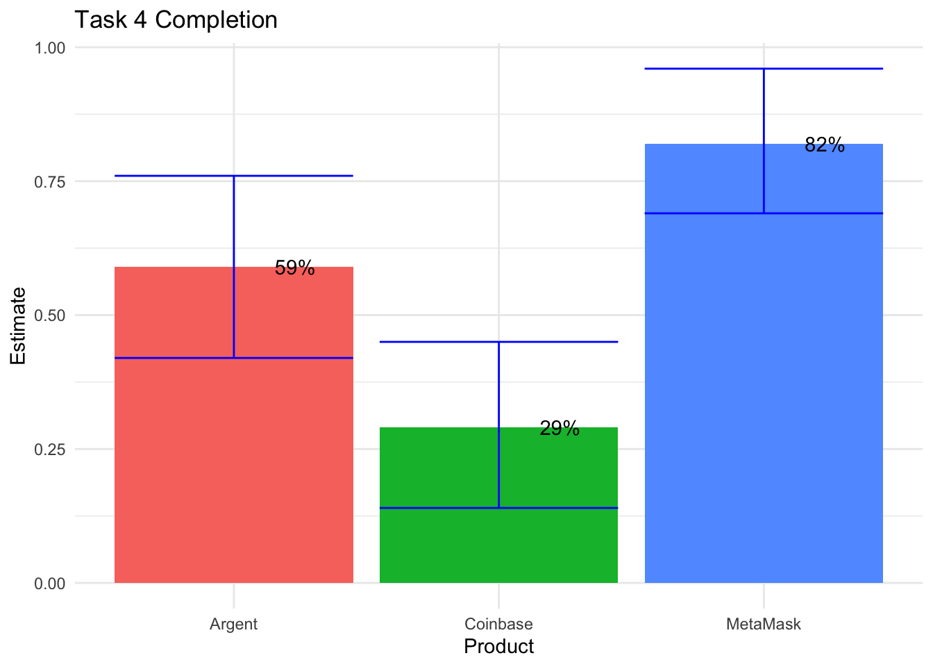
Remember, the Fisher Exact test used above, on the 3x2 contingency tables, indicate a significant difference between completion rates in Task 4; however, we don’t know which wallets have different rates than one another. So now we follow up with several pairwise Fisher Exact tests, testing for significant differences between each wallet pair.
## [1] 0.002509272## [1] 0.2147593## [1] 0.1394198The first test shows that MetaMask has a greater completion rate than Coinbase. The second test returns a relatively large p-value, therefore, there is not a significant difference between Argent and MetaMask. And the third test indicates that Argent has a greater completion rate than Coinbase, not at the 95% c.l., but at the 85% confidence level (p-value = .14). Something to note for later. Perhaps, we will decrease our confidence level to 85% so we can show more over- and under-indexing in our final deliverable to stakeholders. Anyways, our takeaways from Task 4 stat testing is: MetaMask = Argent > Coinbase.
Now, let’s visualize the Task 5 completion rates, as well as the confidence intervals.
# Task 5 Completion Visual + CI's
MM <- addz2ci(x = t5[1,1], n = 15, conf.level = .85)
AG <- addz2ci(x = t5[2,1], n = 15, conf.level = .85)
CB <- addz2ci(x = t5[3,1], n = 15, conf.level = .85)

plot.dat <- data.frame(Product = c("MetaMask", "Argent", "Coinbase"),
                       Estimate = c(MM$estimate, AG$estimate, CB$estimate),
                       Lower = c(MM$conf.int[1], AG$conf.int[1], CB$conf.int[1]),
                       Upper = c(MM$conf.int[2], AG$conf.int[2], CB$conf.int[2]))

ggplot(data = plot.dat) + geom_bar(stat = "identity",
                                   aes(x = Product, y = Estimate, fill = Product)) +
        geom_errorbar(aes(x=Product,
        ymin = Lower,
        ymax = Upper), color = "blue") +
        geom_text(aes(x=Product,y=Estimate,
                      label = paste0((round(Estimate,2)*100),"%"), hjust=-1)) +
  labs(title = "Task 5 Completion") + theme_minimal() + theme(legend.position = "none")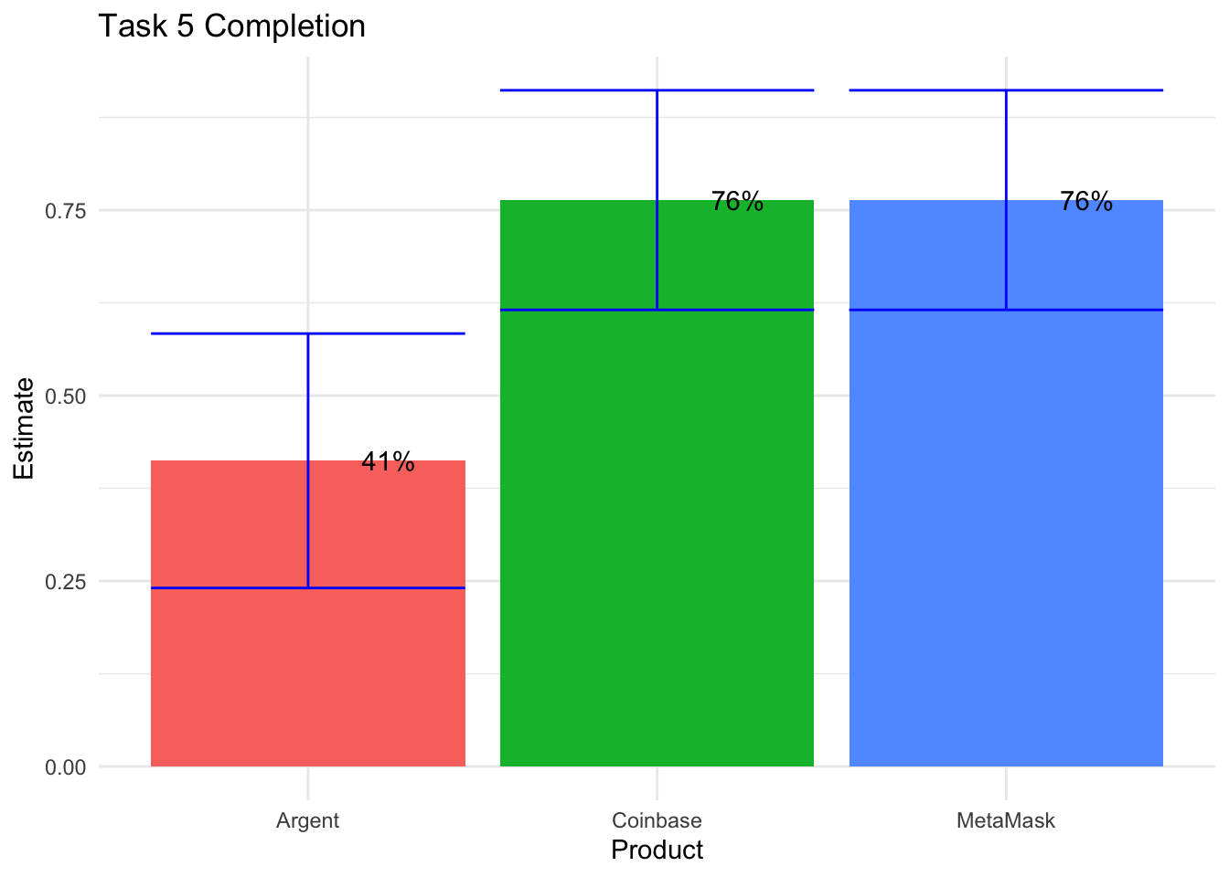
Now, just as we did with Task 4 completion rates, we follow-up with pairwise stat testing on Task 5 completion rates.
## [1] 1## [1] 0.06043294## [1] 0.06043294We see from the first and third test that Coinbase has lower completion rates than both Argent and MetaMask on Task 5, significant at the 94% confidence level (p-value = .06). From here, let’s drop down to the 85% confidence level - significant differences exist at this level, as indicated by the 3x2 Exact Fisher tests that we continue to refer to above, for Tasks 1 and 3. Let’s run visuals for the first three tasks.
# Task 1 Completion Visual + CI's
MM <- addz2ci(x = t1[1,1], n = 15, conf.level = .85)
AG <- addz2ci(x = t1[2,1], n = 15, conf.level = .85)
CB <- addz2ci(x = t1[3,1], n = 15, conf.level = .85)

plot.dat <- data.frame(Product = c("MetaMask", "Argent", "Coinbase"),
                       Estimate = c(MM$estimate, AG$estimate, CB$estimate),
                       Lower = c(MM$conf.int[1], AG$conf.int[1], CB$conf.int[1]),
                       Upper = c(MM$conf.int[2], AG$conf.int[2], CB$conf.int[2]))

plot1 <- ggplot(data = plot.dat) +
  geom_bar(stat = "identity", aes(x = Product,
                                  y = Estimate,
                                  fill = Product)) +
  geom_errorbar(aes(x=Product,
                    ymin = Lower,
                    ymax = Upper),
                color = "blue") +
  geom_text(aes(x=Product,y=Estimate,
                label = paste0((round(Estimate,2)*100),"%"), hjust=-1)) +
  labs(title = "Task 1 Completion") + theme_minimal() + theme(legend.position = "none")


# Task 2 Completion Visual + CI's
MM <- addz2ci(x = t2[1,1], n = 15, conf.level = .85)
AG <- addz2ci(x = t2[2,1], n = 15, conf.level = .85)
CB <- addz2ci(x = t2[3,1], n = 15, conf.level = .85)

plot.dat <- data.frame(Product = c("MetaMask", "Argent", "Coinbase"),
                       Estimate = c(MM$estimate, AG$estimate, CB$estimate),
                       Lower = c(MM$conf.int[1], AG$conf.int[1], CB$conf.int[1]),
                       Upper = c(MM$conf.int[2], AG$conf.int[2], CB$conf.int[2]))

plot2 <- ggplot(data = plot.dat) +
  geom_bar(stat = "identity", aes(x = Product,
                                  y = Estimate,
                                  fill = Product)) +
  geom_errorbar(aes(x=Product,
                    ymin = Lower,
                    ymax = Upper), color = "blue") +
  geom_text(aes(x=Product,y=Estimate,
                label = paste0((round(Estimate,2)*100),"%"), hjust=-1)) +
  labs(title = "Task 2 Completion") + theme_minimal() + theme(legend.position = "none")


# Task 3 Completion Visual + CI's
MM <- addz2ci(x = t3[1,1], n = 15, conf.level = .85)
AG <- addz2ci(x = t3[2,1], n = 15, conf.level = .85)
CB <- addz2ci(x = t3[3,1], n = 15, conf.level = .85)

plot.dat <- data.frame(Product = c("MetaMask", "Argent", "Coinbase"),
                       Estimate = c(MM$estimate, AG$estimate, CB$estimate),
                       Lower = c(MM$conf.int[1], AG$conf.int[1], CB$conf.int[1]),
                       Upper = c(MM$conf.int[2], AG$conf.int[2], CB$conf.int[2]))

plot3 <- ggplot(data = plot.dat) +
  geom_bar(stat = "identity", aes(x = Product,
                                  y = Estimate,
                                  fill = Product)) +
  geom_errorbar(aes(x=Product,
                    ymin = Lower,
                    ymax = Upper), color = "blue") +
  geom_text(aes(x=Product,y=Estimate,
                label = paste0((round(Estimate,2)*100),"%"), hjust=-1)) +
  labs(title = "Task 3 Completion") + theme_minimal() + theme(legend.position = "none")

grid.arrange(plot1, plot2, plot3)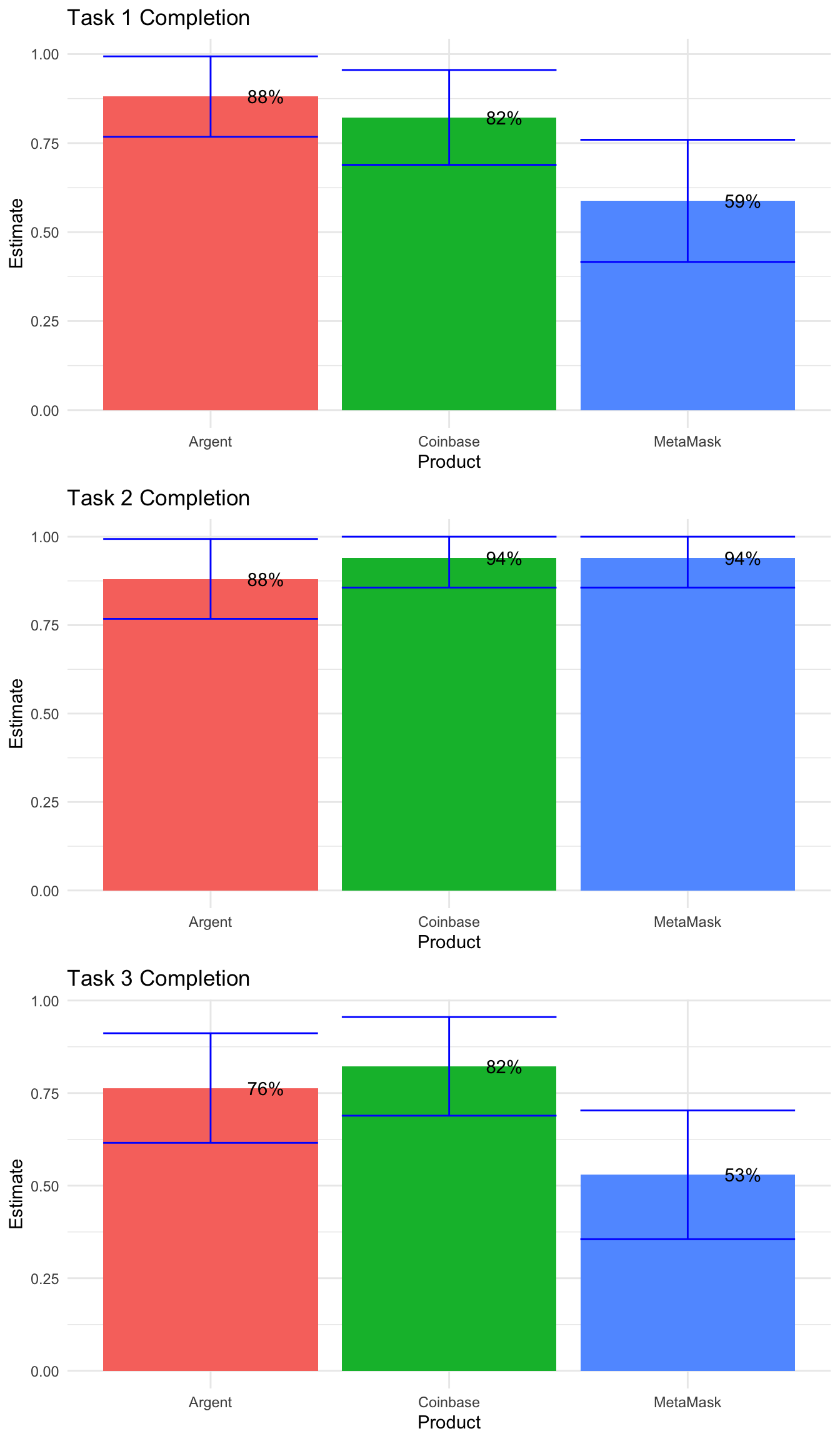
As well as pairwise Fisher Exact tests for the first three tasks.
## [1] 0.2147593## [1] 0.08007663## [1] 1## [1] 1## [1] 1## [1] 1## [1] 0.1086457## [1] 0.2450775## [1] 1As expected, there are no significant differences on Task 2. On Task 1, there are significant differences between Argent and MetaMask. And, on Task 3, there are significant differences between MetaMask and Coinbase. Let’s summarize all of the significance findings, at the 85% confidence level, by task.
- Task 1
Coinbase = Argent > MetaMask (at 89% c.l.)
- Task 2
None
- Task 3
Argent = Coinbase > MetaMask (at 92% c.l.)
- Task 4
MetaMask > Coinbase (at 97% c.l.) & Argent > Coinbase (at 86% c.l.)
- Task 5
Coinbase = MetaMask > Argent (at 94% c.l.)
The bar charts are great additions to the appendix, intended for a more detail-oriented audience. We will just show the point estimates, highlighting significant differences between the wallets across the tasks, in the final scorecard deliverable. Sauro recommends using raw point estimates, and not those calculated from the adjusted-Wald tests, when reporting completion rates that generally fall in the 50%-90% range, which ours do (Sauro and Lewis 2016). These raw point estimates are shown below and will appear on the usability scorecard. Next, we move to the other half of our data - the time and SUS variables.
final.prop <- data.frame(Product = c("MetaMask", "Argent", "Coinbase"),
                         T1_Completion = round(c(MM1, AG1, CB1)/15,2),
                         T2_Completion = round(c(MM2, AG2, CB2)/15,2),
                         T3_Completion = round(c(MM3, AG3, CB3)/15,2),
                         T4_Completion = round(c(MM4, AG4, CB4)/15,2),
                         T5_Completion = round(c(MM5, AG5, CB5)/15,2))

final.prop
## Product T1_Completion T2_Completion T3_Completion T4_Completion
## 1 MetaMask 0.60 1.00 0.53 0.87
## 2 Argent 0.93 0.93 0.80 0.60
## 3 Coinbase 0.87 1.00 0.87 0.27
## T5_Completion
## 1 0.8
## 2 0.4
## 3 0.86.3.2 Continuous Data & ANOVA/t-tests
Now that we calculated point estimates, confidence intervals and conducted stat testing on all “completion rates” (binomial variables), let’s now do the same for “time” and “SUS” (continuous variables). These are slightly easier to handle, using a technique called “analysis of variance” (ANOVA). ANOVA compares the means of 3 or more groups at once, and indicates whether or not there is a difference between at least two groups, or wallets in our case.
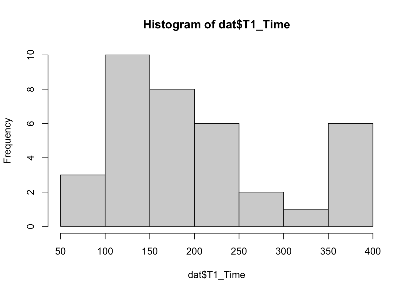
Before we apply ANOVA, we need to transform the “time” variables. Task times have positively skewed distributions as seen in the histogram below. It shows a right-tail of longer times, which skew the average and exert undue influence on the mean. To mitigate this Sauro recommends using geometric mean for “time on task” point estimates on small sample sizes (<26n), and median for larger sample sizes (26n+) (Sauro and Lewis 2016).
Geometric means are calculated by log-transforming the task times, taking the mean of these transformed values, then exponentiating this mean. Thus, we call a t-test on log transformed data in order to obtain our point estimate (i.e. geometric mean) and the proper confidence intervals. We do not do this for SUS, because it does not suffer from skew. Instead we use the regular mean as the point estimate for SUS.
By the way, we use t.tests below to calculate these confidence intervals. We will utilize t.tests later on for the pairwise stat testing of continuous variables, after we run ANOVA tests.
#MetaMask
MM1 <- log(dat[dat[,"User"] == "MetaMask","T1_Time"])
MM1 <- t.test(MM1, conf.level = .85)

MM2 <- log(dat[dat[,"User"] == "MetaMask","T2_Time"])
MM2 <- t.test(MM2, conf.level = .85)

MM3 <- log(dat[dat[,"User"] == "MetaMask","T3_Time"])
MM3 <- t.test(MM3, conf.level = .85)

MM4 <- log(dat[dat[,"User"] == "MetaMask","T4_Time"])
MM4 <- t.test(MM4, conf.level = .85)

MM5 <- log(dat[dat[,"User"] == "MetaMask","T5_Time"])
MM5 <- t.test(MM5, conf.level = .85)

MM.sus <- dat[dat[,"User"] == "MetaMask","SUS"]
MM.sus <- t.test(MM.sus)

#Argent
AG1 <- log(dat[dat[,"User"] == "Argent","T1_Time"])
AG1 <- t.test(AG1, conf.level = .85)

AG2 <- log(dat[dat[,"User"] == "Argent","T2_Time"])
AG2 <- t.test(AG2, conf.level = .85)

AG3 <- log(dat[dat[,"User"] == "Argent","T3_Time"])
AG3 <- t.test(AG3, conf.level = .85)

AG4 <- log(dat[dat[,"User"] == "Argent","T4_Time"])
AG4 <- t.test(AG4, conf.level = .85)

AG5 <- log(dat[dat[,"User"] == "Argent","T5_Time"])
AG5 <- t.test(AG5, conf.level = .85)

AG.sus <- dat[dat[,"User"] == "Argent","SUS"]
AG.sus <- t.test(AG.sus)

#Coinbase
CB1 <- log(dat[dat[,"User"] == "Coinbase","T1_Time"])
CB1 <- t.test(CB1, conf.level = .85)

CB2 <- log(dat[dat[,"User"] == "Coinbase","T2_Time"])
CB2 <- t.test(CB2, conf.level = .85)

CB3 <- log(dat[dat[,"User"] == "Coinbase","T3_Time"])
CB3 <- t.test(CB3, conf.level = .85)

CB4 <- log(dat[dat[,"User"] == "Coinbase","T4_Time"])
CB4 <- t.test(CB4, conf.level = .85)

CB5 <- log(dat[dat[,"User"] == "Coinbase","T5_Time"])
CB5 <- t.test(CB5, conf.level = .85)

CB.sus <- dat[dat[,"User"] == "Coinbase","SUS"]
CB.sus <- t.test(CB.sus)
And just like with the binary variables in the previous section, we visualize all the continuous variables, charting point estimates on the y-axis as well as confidence intervals.
# Task 1
plot.dat <- data.frame(Product = c("MetaMask", "Argent", "Coinbase"),
                       Estimate = c(exp(MM1$estimate), exp(AG1$estimate), exp(CB1$estimate)),
                       Lower = c(exp(MM1$conf.int[1]), exp(AG1$conf.int[1]), exp(CB1$conf.int[1])),
                       Upper = c(exp(MM1$conf.int[2]), exp(AG1$conf.int[2]), exp(CB1$conf.int[2])))

plot1 <- ggplot(data = plot.dat) +
  geom_bar(stat = "identity", aes(x = Product,
                                  y = Estimate,
                                  fill = Product)) +
  geom_errorbar(aes(x=Product,
                    ymin = Lower,
                    ymax = Upper), color = "blue") +
  geom_text(aes(x=Product,y=Estimate,
                label = round(Estimate,0), hjust=0)) +
  labs(title = "Task 1 Time") + theme_minimal() + theme(legend.position = "none")

# Task 2
plot.dat <- data.frame(Product = c("MetaMask", "Argent", "Coinbase"),
                       Estimate = c(exp(MM2$estimate), exp(AG2$estimate), exp(CB2$estimate)),
                       Lower = c(exp(MM2$conf.int[1]), exp(AG2$conf.int[1]), exp(CB2$conf.int[1])),
                       Upper = c(exp(MM2$conf.int[2]), exp(AG2$conf.int[2]), exp(CB2$conf.int[2])))

plot2 <- ggplot(data = plot.dat) +
  geom_bar(stat = "identity", aes(x = Product,
                                  y = Estimate,
                                  fill = Product)) +
  geom_errorbar(aes(x=Product,
                    ymin = Lower,
                    ymax = Upper), color = "blue") +
  geom_text(aes(x=Product,y=Estimate,
                label = round(Estimate,0), hjust=0)) +
  labs(title = "Task 2 Time") + theme_minimal() + theme(legend.position = "none")

# Task 3
plot.dat <- data.frame(Product = c("MetaMask", "Argent", "Coinbase"),
                       Estimate = c(exp(MM3$estimate), exp(AG3$estimate), exp(CB3$estimate)),
                       Lower = c(exp(MM3$conf.int[1]), exp(AG3$conf.int[1]), exp(CB3$conf.int[1])),
                       Upper = c(exp(MM3$conf.int[2]), exp(AG3$conf.int[2]), exp(CB3$conf.int[2])))

plot3 <- ggplot(data = plot.dat) +
  geom_bar(stat = "identity", aes(x = Product,
                                  y = Estimate,
                                  fill = Product)) +
  geom_errorbar(aes(x=Product,
                    ymin = Lower,
                    ymax = Upper), color = "blue") +
  geom_text(aes(x=Product,y=Estimate,
                label = round(Estimate,0), hjust=0)) +
  labs(title = "Task 3 Time") + theme_minimal() + theme(legend.position = "none")

# Task 4
plot.dat <- data.frame(Product = c("MetaMask", "Argent", "Coinbase"),
                       Estimate = c(exp(MM4$estimate), exp(AG4$estimate), exp(CB4$estimate)),
                       Lower = c(exp(MM4$conf.int[1]), exp(AG4$conf.int[1]), exp(CB4$conf.int[1])),
                       Upper = c(exp(MM4$conf.int[2]), exp(AG4$conf.int[2]), exp(CB4$conf.int[2])))

plot4 <- ggplot(data = plot.dat) +
  geom_bar(stat = "identity", aes(x = Product,
                                  y = Estimate,
                                  fill = Product)) +
  geom_errorbar(aes(x=Product,
                    ymin = Lower,
                    ymax = Upper), color = "blue") +
  geom_text(aes(x=Product,y=Estimate,
                label = round(Estimate,0), hjust=0)) +
  labs(title = "Task 4 Time") + theme_minimal() + theme(legend.position = "none")

# Task 5
plot.dat <- data.frame(Product = c("MetaMask", "Argent", "Coinbase"),
                       Estimate = c(exp(MM5$estimate), exp(AG5$estimate), exp(CB5$estimate)),
                       Lower = c(exp(MM5$conf.int[1]), exp(AG5$conf.int[1]), exp(CB5$conf.int[1])),
                       Upper = c(exp(MM5$conf.int[2]), exp(AG5$conf.int[2]), exp(CB5$conf.int[2])))

plot5 <- ggplot(data = plot.dat) +
  geom_bar(stat = "identity", aes(x = Product,
                                  y = Estimate,
                                  fill = Product)) +
  geom_errorbar(aes(x=Product,
                    ymin = Lower,
                    ymax = Upper), color = "blue") +
  geom_text(aes(x=Product,y=Estimate,
                label = round(Estimate,0), hjust=0)) +
  labs(title = "Task 5 Time") + theme_minimal() + theme(legend.position = "none")

#SUS
plot.dat <- data.frame(Product = c("MetaMask", "Argent", "Coinbase"),
                       Estimate = c(MM.sus$estimate, AG.sus$estimate, CB.sus$estimate),
                       Lower = c(MM.sus$conf.int[1], AG.sus$conf.int[1], CB.sus$conf.int[1]),
                       Upper = c(MM.sus$conf.int[2], AG.sus$conf.int[2], CB.sus$conf.int[2]))

plot6 <- ggplot(data = plot.dat) +
  geom_bar(stat = "identity", aes(x = Product,
                                  y = Estimate,
                                  fill = Product)) +
  geom_errorbar(aes(x=Product,
                    ymin = Lower,
                    ymax = Upper), color = "blue") +
  geom_text(aes(x=Product,y=Estimate,
                label = round(Estimate,0), hjust=0)) +
  labs(title = "System Usability Score") +
  theme_minimal() +
  theme(legend.position = "none")

grid.arrange(plot1, plot2, plot3, plot4, plot5, plot6)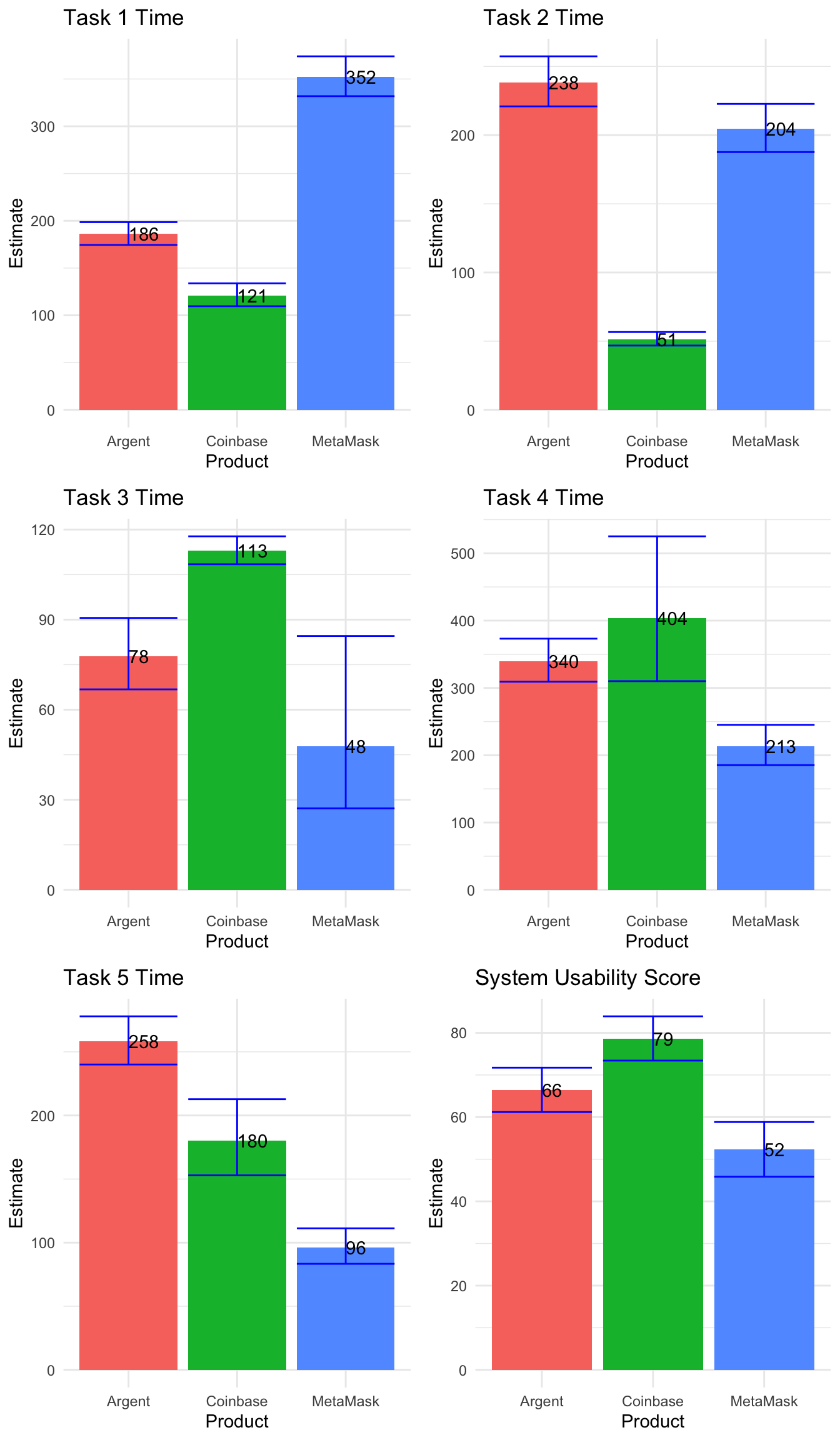
Visually, we see differences between these means, but we come back to the same question: do these differences really exist in the population, or are they just attributed to noise in our sample? We answer this first with an ANOVA test, then move to pairwise comparisons (using t.tests) to test relationships between wallet pairs. If you remember, this is the exact same process we followed in the previous section - group-level tests followed by pairwise tests.
## Analysis of Variance Table
##
## Response: T1_Time
##           Df  Sum Sq Mean Sq F value    Pr(>F)
## dat$User   3 1825589  608530  634.77 < 2.2e-16 ***
## Residuals 33   31636     959
## ---
## Signif. codes: 0 '***' 0.001 '**' 0.01 '*' 0.05 '.' 0.1 ' ' 1## Analysis of Variance Table
##
## Response: T2_Time
## Df Sum Sq Mean Sq F value Pr(>F)
## dat$User 3 1515430 505143 440.53 < 2.2e-16 ***
## Residuals 41 47014 1147
## ---
## Signif. codes: 0 '***' 0.001 '**' 0.01 '*' 0.05 '.' 0.1 ' ' 1## Analysis of Variance Table
##
## Response: T3_Time
## Df Sum Sq Mean Sq F value Pr(>F)
## dat$User 3 278438 92813 184 < 2.2e-16 ***
## Residuals 30 15132 504
## ---
## Signif. codes: 0 '***' 0.001 '**' 0.01 '*' 0.05 '.' 0.1 ' ' 1## Analysis of Variance Table
##
## Response: T4_Time
## Df Sum Sq Mean Sq F value Pr(>F)
## dat$User 3 2401616 800539 160.35 1.474e-15 ***
## Residuals 23 114823 4992
## ---
## Signif. codes: 0 '***' 0.001 '**' 0.01 '*' 0.05 '.' 0.1 ' ' 1## Analysis of Variance Table
##
## Response: T5_Time
## Df Sum Sq Mean Sq F value Pr(>F)
## dat$User 3 963260 321087 153.78 < 2.2e-16 ***
## Residuals 27 56376 2088
## ---
## Signif. codes: 0 '***' 0.001 '**' 0.01 '*' 0.05 '.' 0.1 ' ' 1## Analysis of Variance Table
##
## Response: SUS
## Df Sum Sq Mean Sq F value Pr(>F)
## dat$User 3 200176 66725 629.14 < 2.2e-16 ***
## Residuals 42 4454 106
## ---
## Signif. codes: 0 '***' 0.001 '**' 0.01 '*' 0.05 '.' 0.1 ' ' 1The ANOVA tests, with their small p-values, indicate that significant differences exist on all continuous variables. Thus, we follow-up with pairwise t.tests.
##
##  Pairwise comparisons using t tests with pooled SD
##
## data:  dat$T1_Time and dat$User
##
##          Argent  Coinbase
## Coinbase 6.2e-06 -
## MetaMask 4.1e-14 < 2e-16
##
## P value adjustment method: none##
## Pairwise comparisons using t tests with pooled SD
##
## data: dat$T2_Time and dat$User
##
## Argent Coinbase
## Coinbase < 2e-16 -
## MetaMask 0.011 1.1e-15
##
## P value adjustment method: none##
## Pairwise comparisons using t tests with pooled SD
##
## data: dat$T3_Time and dat$User
##
## Argent Coinbase
## Coinbase 0.0013 -
## MetaMask 0.0755 2.1e-05
##
## P value adjustment method: none##
## Pairwise comparisons using t tests with pooled SD
##
## data: dat$T4_Time and dat$User
##
## Argent Coinbase
## Coinbase 0.11067 -
## MetaMask 0.00059 8.4e-05
##
## P value adjustment method: none##
## Pairwise comparisons using t tests with pooled SD
##
## data: dat$T5_Time and dat$User
##
## Argent Coinbase
## Coinbase 0.0057 -
## MetaMask 1.8e-07 4.9e-05
##
## P value adjustment method: none##
## Pairwise comparisons using t tests with pooled SD
##
## data: dat$SUS and dat$User
##
## Argent Coinbase
## Coinbase 0.00231 -
## MetaMask 0.00052 1.4e-08
##
## P value adjustment method: noneAnd all p-values, for the pairwise tests, are below .15, which indicates that all “task times” are significantly different from one wallet to the next, at the 85% confidence level. The final point estimates are printed below for the continuous variables. Remember that we use geometric mean as the point estimate for “task times”. Also, the system usability scores (SUS’s) are significantly different between the wallets (Coinbase > Argent > MetaMask).
final.mean <- data.frame(Product = c("MetaMask", "Argent", "Coinbase"),
                         T1_Time = round(c(exp(MM1$estimate[[1]]),
                                           exp(AG1$estimate[[1]]),
                                           exp(CB1$estimate[[1]])),0),
                         T2_Time = round(c(exp(MM2$estimate[[1]]),
                                           exp(AG2$estimate[[1]]),
                                           exp(CB2$estimate[[1]])),0),
                         T3_Time = round(c(exp(MM3$estimate[[1]]),
                                           exp(AG3$estimate[[1]]),
                                           exp(CB3$estimate[[1]])),0),
                         T4_Time = round(c(exp(MM4$estimate[[1]]),
                                           exp(AG4$estimate[[1]]),
                                           exp(CB4$estimate[[1]])),0),
                         T5_Time = round(c(exp(MM5$estimate[[1]]),
                                           exp(AG5$estimate[[1]]),
                                           exp(CB5$estimate[[1]])),0),
                         SUS = round(c(MM.sus$estimate,
                                     AG.sus$estimate,
                                     CB.sus$estimate),0))

final.mean
## Product T1_Time T2_Time T3_Time T4_Time T5_Time SUS
## 1 MetaMask 352 204 48 213 96 52
## 2 Argent 186 238 78 340 258 66
## 3 Coinbase 121 51 113 404 180 79We print the point estimates for all continuous variables above. This is what we use for the final scorecard, and since all are significantly different from each other at the 85% c.l., we can indicate greatest to least performance for each task.
6.4 Conclusion
The final usability scorecard is shown below. It includes point estimates for completion rate and task time for each task, as well as point estimates for the system usability score (SUS). These point estimates are compared across the three crypto wallets and statistical significance is marked by colored boxes around the point estimates.
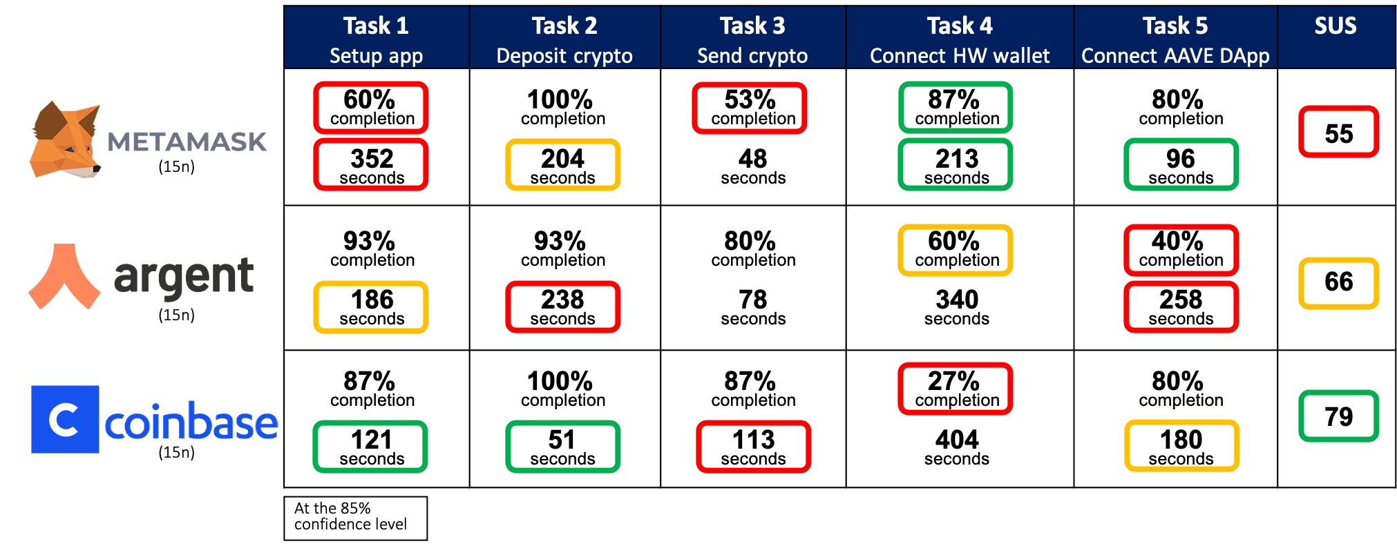
Red means poorest performance, green means best performance, and orange means that it’s middle-of-the-road performance. MetaMask has the greatest completion on Task 4, but the lowest completion on Tasks 1 and 3, and the lowest SUS. Argent has the lowest completion on Task 5, and a middle-of-the-road SUS. Finally, Coinbase has the lowest completion on Task 4, but relatively high completion on the other tasks, as well as the highest SUS. This performance comparison indicates to product managers of the respective apps which areas to focus their UX improvements.
Also, once the product has been redesigned and improved, it can be retested in similar conditions, with similar sample, and these point estimates can be carried over and used as benchmark metrics. Tracking usability metrics in this way gives product teams an objective means of validating design changes and measuring improvement, stagnation, or degradation of the product’s user experience.
Bibliography
Budiu, R. 2018. “Between-Subjects Vs. Within-Subjects Study Design.” Nielsen Norman Group. https://www.nngroup.com/articles/between-within-subjects/.
Chapman, C, and E Feit. 2019. R for Marketing Research and Analytics. New York, NY: Springer Berlin Heidelberg.
Joyce, A. 2019. “Formative Vs. Summative Evaluations.” Nielsen Norman Group. https://www.nngroup.com/articles/formative-vs-summative-evaluations/.
Sauro, Jeff, and James R. Lewis. 2016. Quantifying the User Experience: Practical Statistics for User Research. 2nd edition. Cambridge: Morgan Kaufmann.
Särndal, Carl-Erik, Bengt Swensson, Jan Håkan Wretman, and Särndal-Swensson-Wretman. 2003. Model Assisted Survey Sampling. 1. softcover print. Springer Series in Statistics. New York, NY: Springer.
Tullis, Tom, and Bill Albert. 2013. Measuring the User Experience: Collecting, Analyzing, and Presenting Usability Metrics. Second edition. Amsterdam ; Boston: Elsevier/Morgan Kaufmann.