第 5 章 Annotation and Maps

5.1 地圖基本元素

多由point, line, polygon(多邊體)組成。

• point: 如景點位置；geom_point

• line: 如河流； geom_path

• polygon: 如臺北市範圍界線；geom_polygon

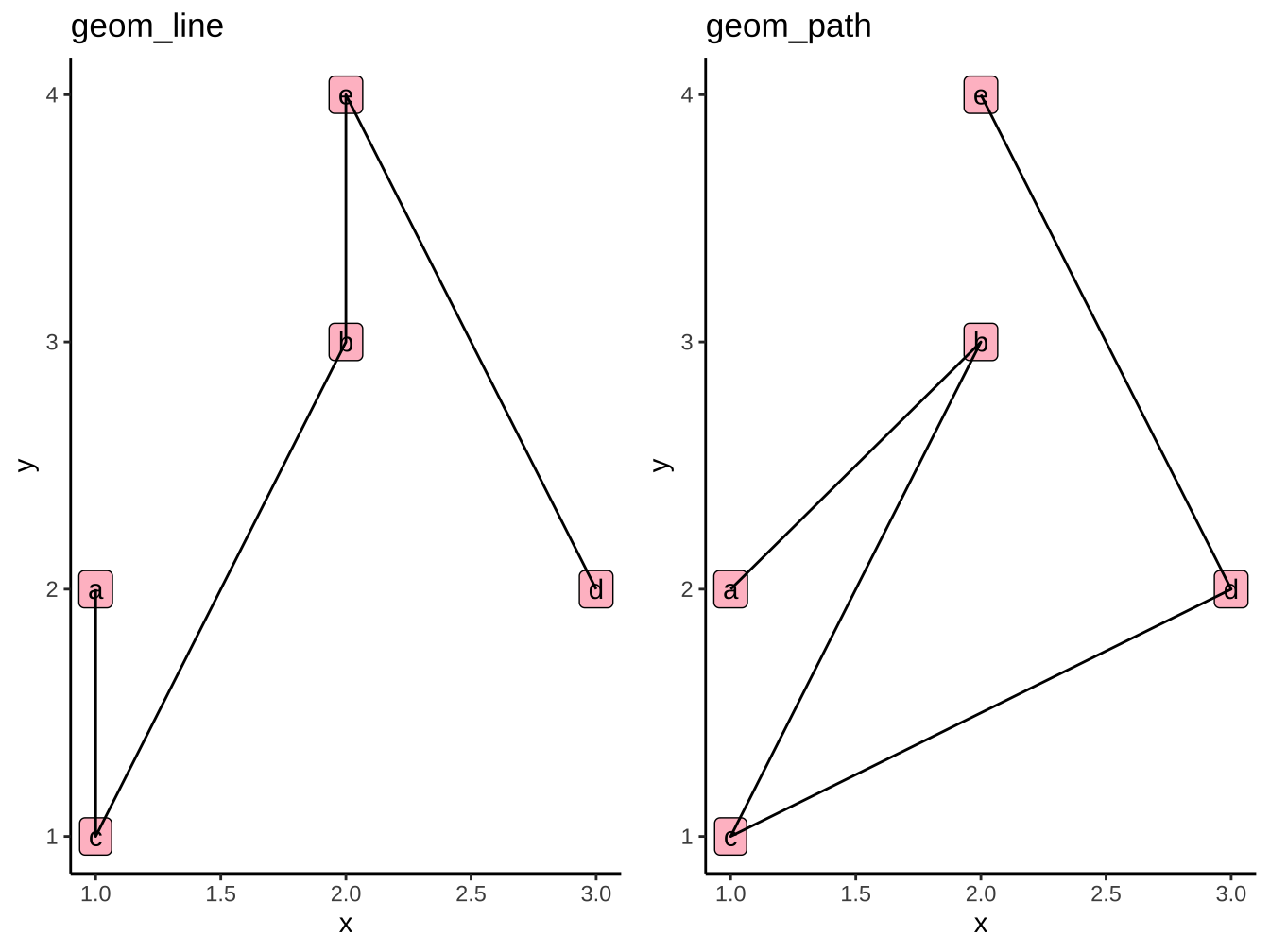
geom_line與geom_path差異在：

• geom_line: 以x值排序繪成。

• geom_path: 以(x,y)出現順序繪成。

df0 <- data.frame(
  x=c(1,2,1,3,2),
  y=c(2,3,1,2,4),
  label=c("a","b","c","d","e")
)
df0 %>%
  ggplot(aes(x=x,y=y))+
  geom_label(
    aes(label=label), fill="pink"
    )-> plotbase0

list_graphs <- list()

plotbase0+geom_line()+labs(title="geom_line") -> 
  list_graphs$geom_line

plotbase0+geom_path()+labs(title="geom_path") -> 
  list_graphs$geom_path

ggpubr::ggarrange(
  list_graphs$geom_line, list_graphs$geom_path
)

5.1.1 Point, line, polygon

為方便說明，先創造格線底圖myGrids：

ggplot()+theme_linedraw()+
  scale_x_continuous(limits=c(0,6),breaks=0:6,
                     expand=expand_scale(add=c(0,0)))+
  scale_y_continuous(limits=c(0,6),breaks=0:6,
                     expand=expand_scale(mult = c(0,0))) ->
  myGrids

myGrids

• theme_linedraw(): 圖面每個breaks均有格線
  
• expand=…: 用來設定在資料limits上限及下限要再延伸多少.
  expand_scale(add=c(a1,a2)) 下限減a1，上限加a2；或 expand_scale(mult=c(m1,m2)) 下限減limits長度m1倍，上限加其m2倍。

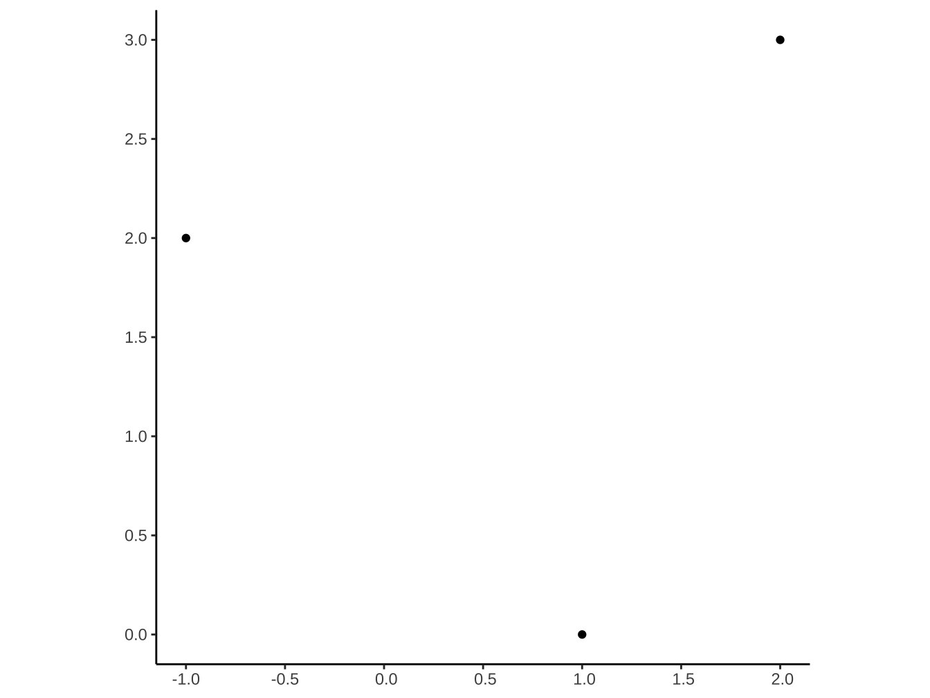
5.1.2 Matrix expression

後面介紹到地圖常用的simple features時，因其格式多以矩陣方式輸入，故在此也用矩陣說明。

用rbind()產生\(4\times 2\)矩陣，代表在xy平面的三個點：

list_geometryData <- list()
list_geometryData$points <- 
  rbind(
    c(1,5),
    c(2,1),
    c(5,1),
    c(5,5)) 

矩陣as.data.frame後，會形成V1, V2名稱欄位。

list_geometryData$points %>%
  as.data.frame() 

V1 V2 1 1 5 2 2 1 3 5 1 4 5 5

myGrids +
  geom_point(
    data=as.data.frame(list_geometryData$points),
    aes(x=V1,y=V2)
  ) -> list_graphs$point

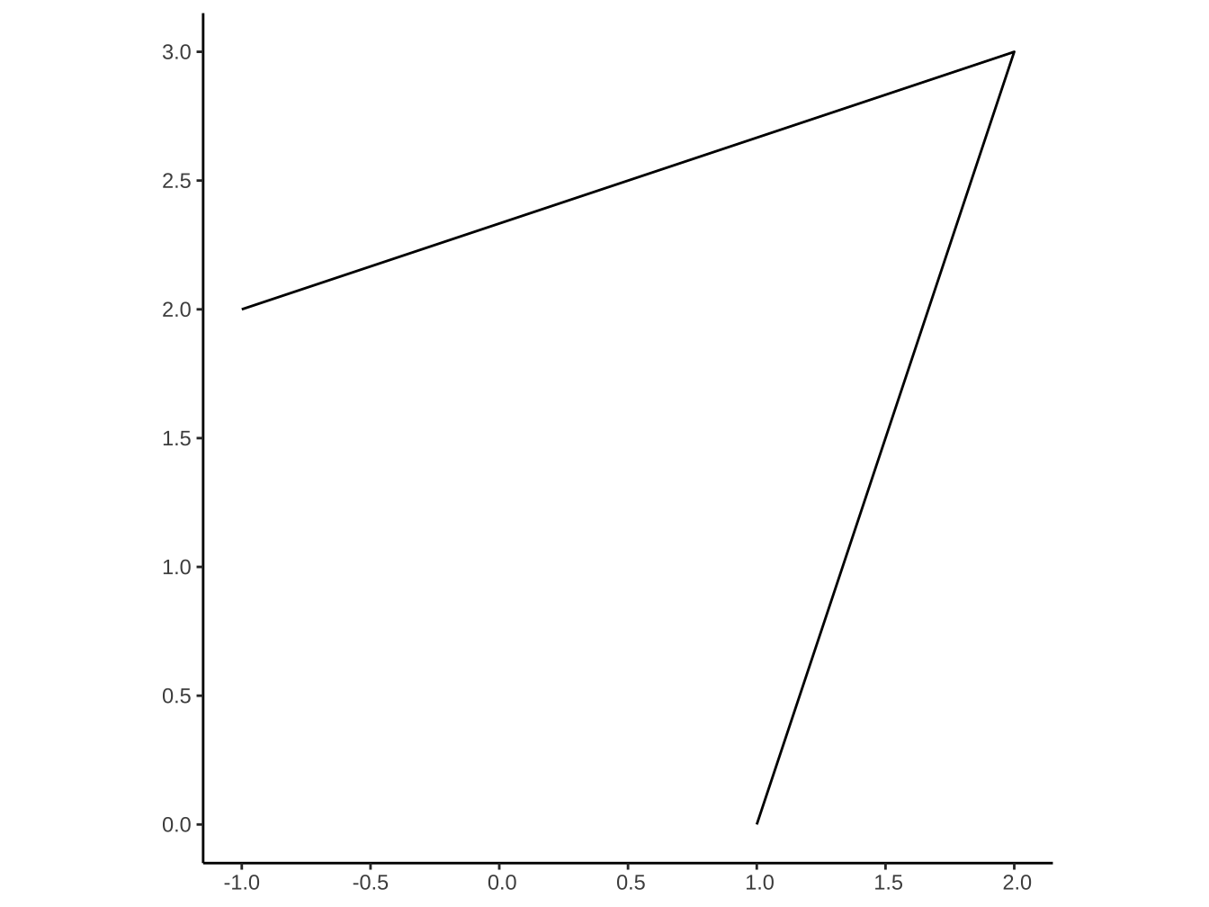
myGrids +
  geom_path(
    data=as.data.frame(list_geometryData$points),
    aes(x=V1,y=V2)
  ) -> list_graphs$path

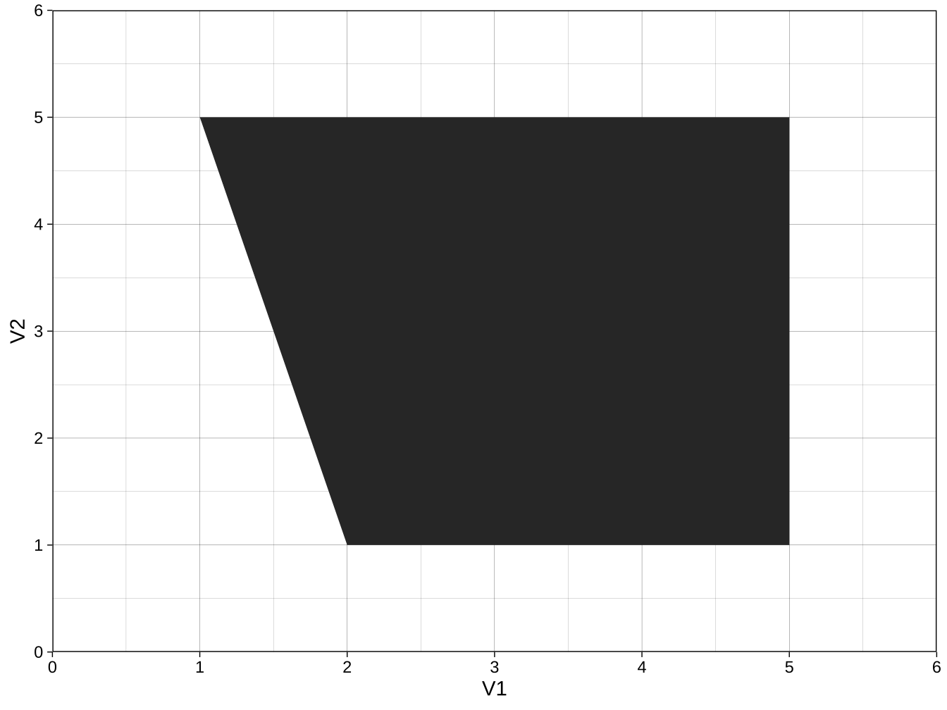
myGrids +
  geom_polygon(
    data=as.data.frame(list_geometryData$points),
    aes(x=V1,y=V2)
  ) -> list_graphs$polygon

ggpubr::ggarrange(
  list_graphs$point, list_graphs$path, list_graphs$polygon,
  ncol=3
)

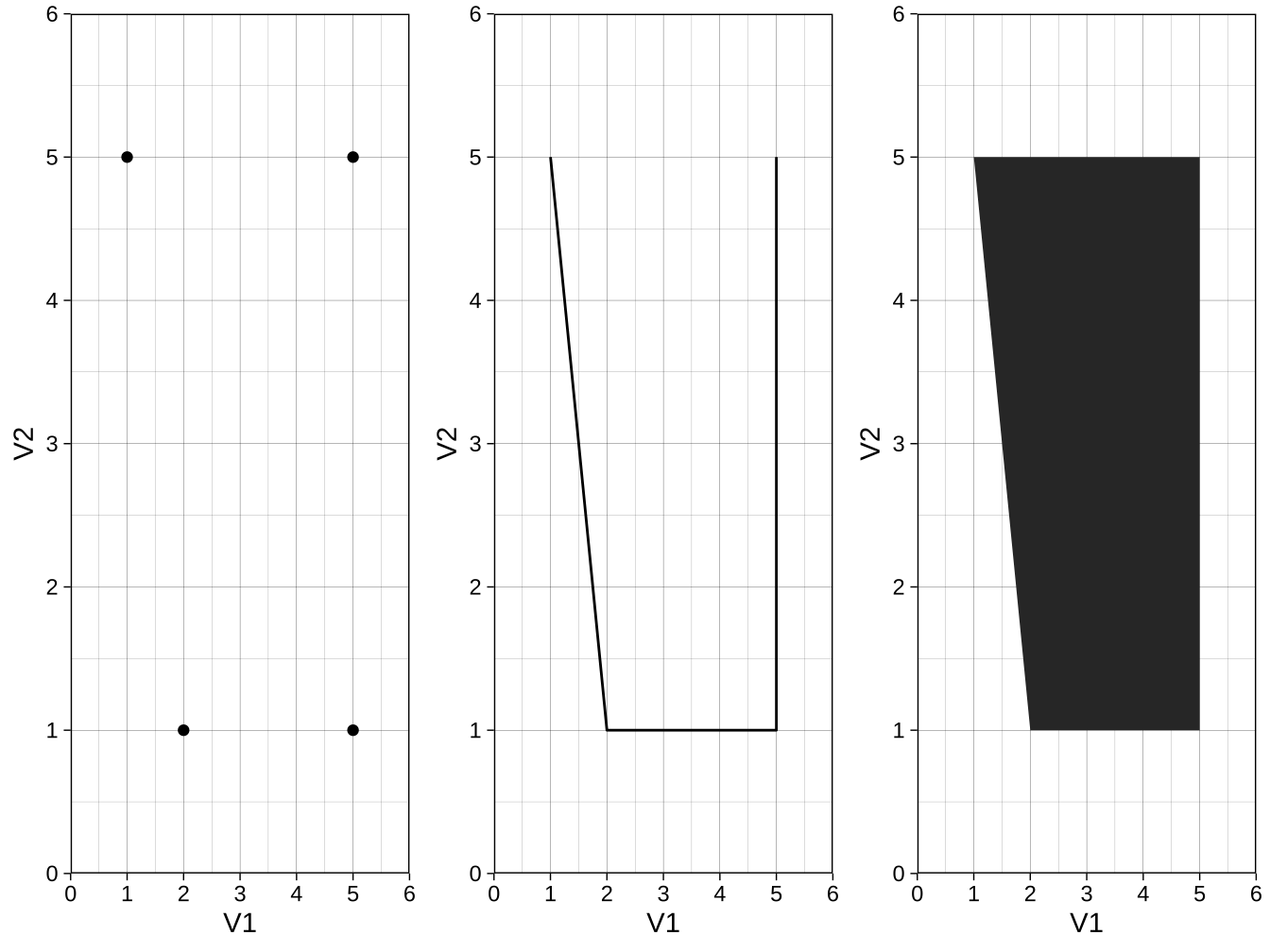
地圖資料中的point, line, polygon便是一系列由：

• 矩陣

• geom

來代表的資訊。

5.1.3 北台灣範例

讀入北台北灣資料：

library(readr)
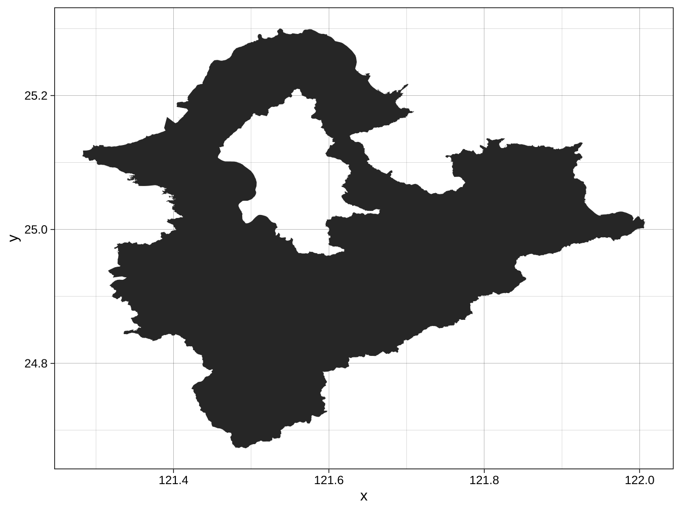
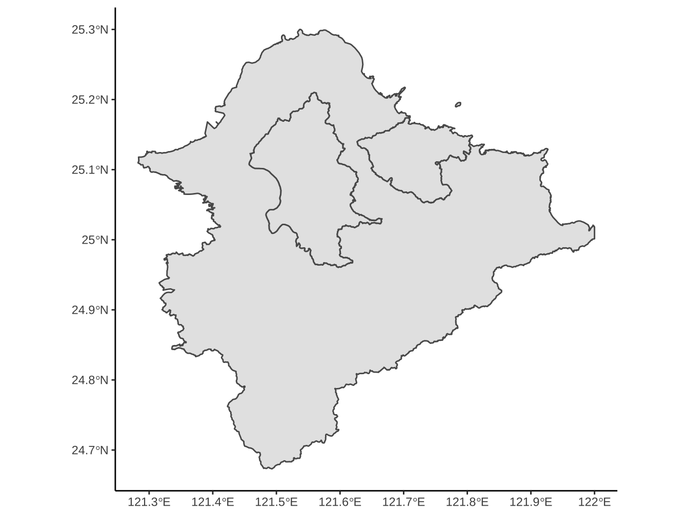
df_geo_northTW <- read_csv("https://www.dropbox.com/s/6uljw24zkyj7avs/df_geo_northTW.csv?dl=1")

選出COUNTYNAME為“新北市”以geom_polygon繪出如下形狀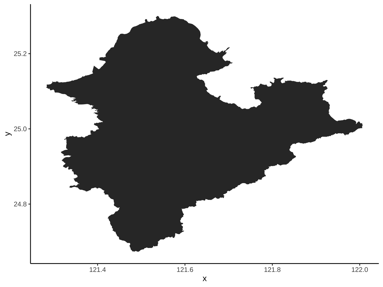： 這張圖新北市地圖有什麼問題？

5.1.4 Polygon with holes

list_graphs$polygon

list_geometryData$hole <-
  rbind(
    c(2,4),
    c(3,2),
    c(4,3)
  )

list_graphs$twoPolygons <-
  list_graphs$polygon+
  geom_polygon(
    data=as.data.frame(list_geometryData$hole),
    aes(x=V1,y=V2), fill="white"
  )

ggpubr::ggarrange(
  list_graphs$polygon, list_graphs$twoPolygons
)

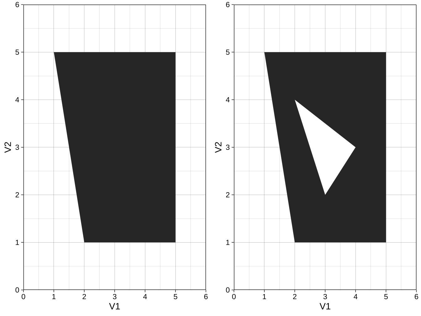
• 這是假像的解決問題，洞並沒有透出底部格線。

list_geometryData$points %>%
  as.data.frame() -> df_part1
list_geometryData$hole %>%
  as.data.frame() -> df_part2

df_part1 %>%
  mutate(
    sub_id=1
  ) -> df_part1

df_part2 %>%
  mutate(
    sub_id=2
  ) -> df_part2

bind_rows(
  df_part1,
  df_part2
) -> df_all

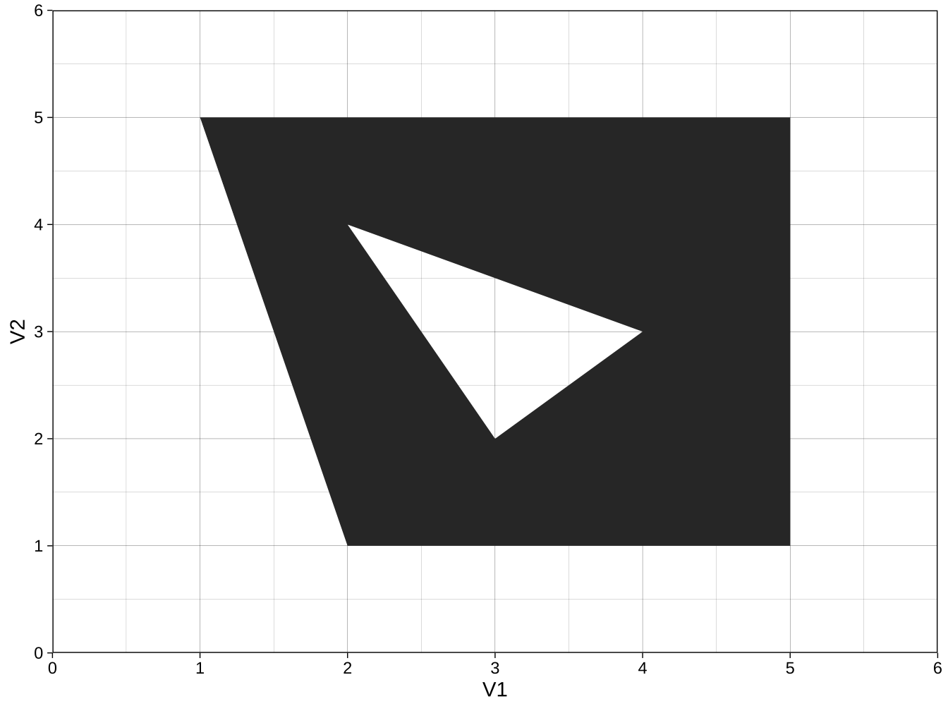
df_all %>%
  mutate(
    group_id="A"
  ) -> df_all

myGrids +
  geom_polygon(
    data=df_all,
    aes(x=V1,y=V2, group=group_id, subgroup=sub_id)
  )

df_all %>%
  add_row(
    V1=c(4,4.5,4.5),
    V2=c(1.5,1.5,2),
    sub_id=c(3,3,3),
    group_id="A"
  ) -> df_all3Subgroups

myGrids+
  geom_polygon(
    data=df_all3Subgroups,
    aes(
      x=V1,y=V2,group=group_id, subgroup=sub_id
    )
  )

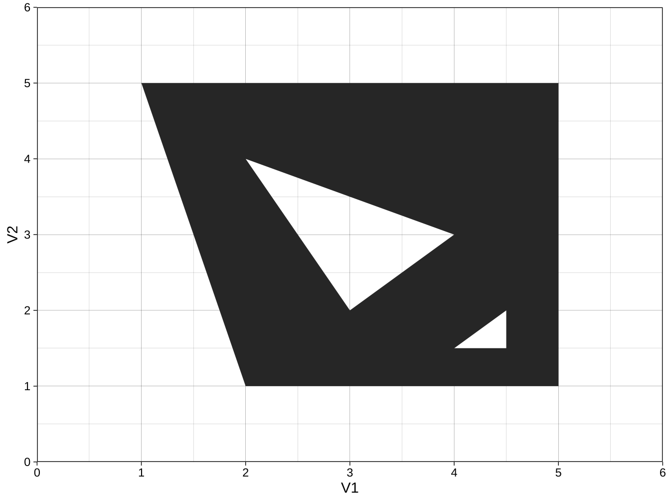
geom_polygon習慣以subgroup的第一群為含蓋地理區塊，以後的都是holes。但實際應用它會去看誰的polygon邊界在最外圍，最外圍的自然不會是hole，而是outer area。

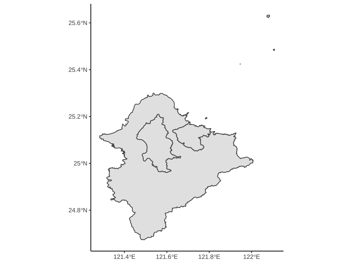
請繪出如下正確的新北市地形圖。

5.1.5 Multipolygons

• 使用aes fill用顏色區分polygons

• color決定邊界線顏色

df_geo_northTW %>%
  ggplot()+
  geom_polygon(
    aes(x=x,y=y,fill=COUNTYNAME), color="azure4"
  ) -> list_graphs$northTW
list_graphs$northTW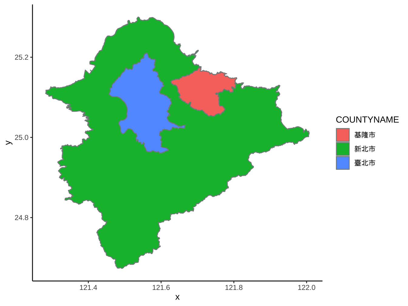

5.2 Annotation

annotate(geom, x = NULL, y = NULL, xmin = NULL, xmax = NULL,
  ymin = NULL, ymax = NULL, xend = NULL, yend = NULL, ...,
  na.rm = FALSE)

• 說明：https://ggplot2.tidyverse.org/reference/annotate.html

5.2.1 線、文字

善用：

• theme_linedraw(): 來決定座標。

• theme_void(): 來得到空白底面。

# load(url("https://www.dropbox.com/s/9n7b1bcs09gnw0r/ggplot_newTaipei.Rda?dl=1")) # 前個練習若沒做出來，執行此行

list_graphs$northTW +
#  theme_linedraw()+
  geom_path(
    data=data.frame(
      x=c(121.55,121.7,121.9),
      y=c(25.1,24.7,24.7)
      ),
    aes(x=x,y=y)
    )+
  annotate(
    "text",
    x=121.9,y=24.71,label="這是臺北市",
    vjust=0
  )+
  theme_void()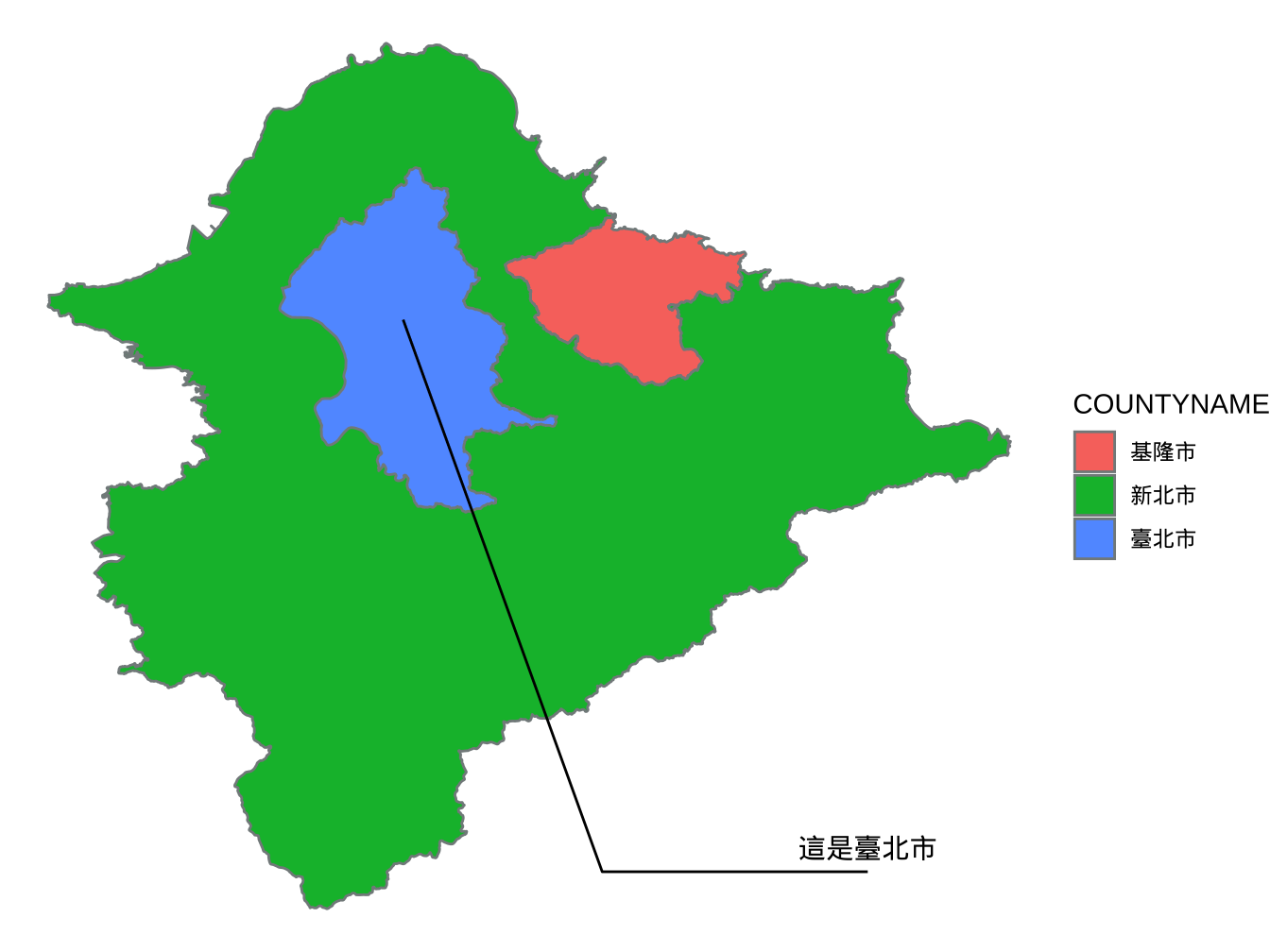

annotate()針對一筆資訊，geom_...()針對多筆資訊使用aes mapping。

5.2.2 圖片

使用annotation_raster():
* 說明： https://ggplot2.tidyverse.org/reference/annotation_raster.html

annotation_raster(raster, xmin, xmax, ymin, ymax, interpolate = FALSE)

• 配合magick套件

• 說明：https://cran.r-project.org/web/packages/magick/vignettes/intro.html

library(magick)
# download.file("https://mir-s3-cdn-cf.behance.net/project_modules/max_1200/2450df20386177.562ea7d13f396.jpg",
#               destfile = "taipei101.jpg")
image_read("https://mir-s3-cdn-cf.behance.net/project_modules/max_1200/2450df20386177.562ea7d13f396.jpg") -> taipei101

查看圖片資訊

taipei101 %>%
  image_info() -> taipei101info
# taipei101info

# 檢視圖片高寬比
taipei101info$height/taipei101info$width -> img_asp # image aspect ratio
img_asp

[1] 0.8571

圖片width,height

ggplot()+theme_linedraw()+
  theme(
    panel.background = element_rect(fill="cyan4")
  )

theme_linedraw()+
  theme(
    panel.background = element_rect(fill="cyan4")
  ) -> list_graphs$theme_backgroundCheck

# 圖片底色非透明
taipei101 %>%
  image_ggplot()+
  list_graphs$theme_backgroundCheck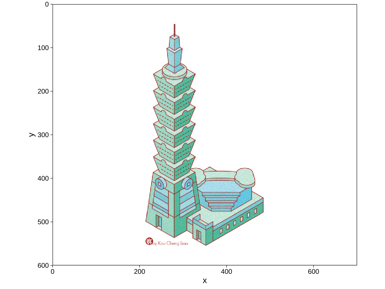

圖片填色（讓背景為透明） point=“++”; 小心y軸0在上方。

image_fill(taipei101, "transparent", point = "+100+100", fuzz = 0) %>% # fuzz=對邊界定義模糊度 %>%
    image_ggplot()+list_graphs$theme_backgroundCheck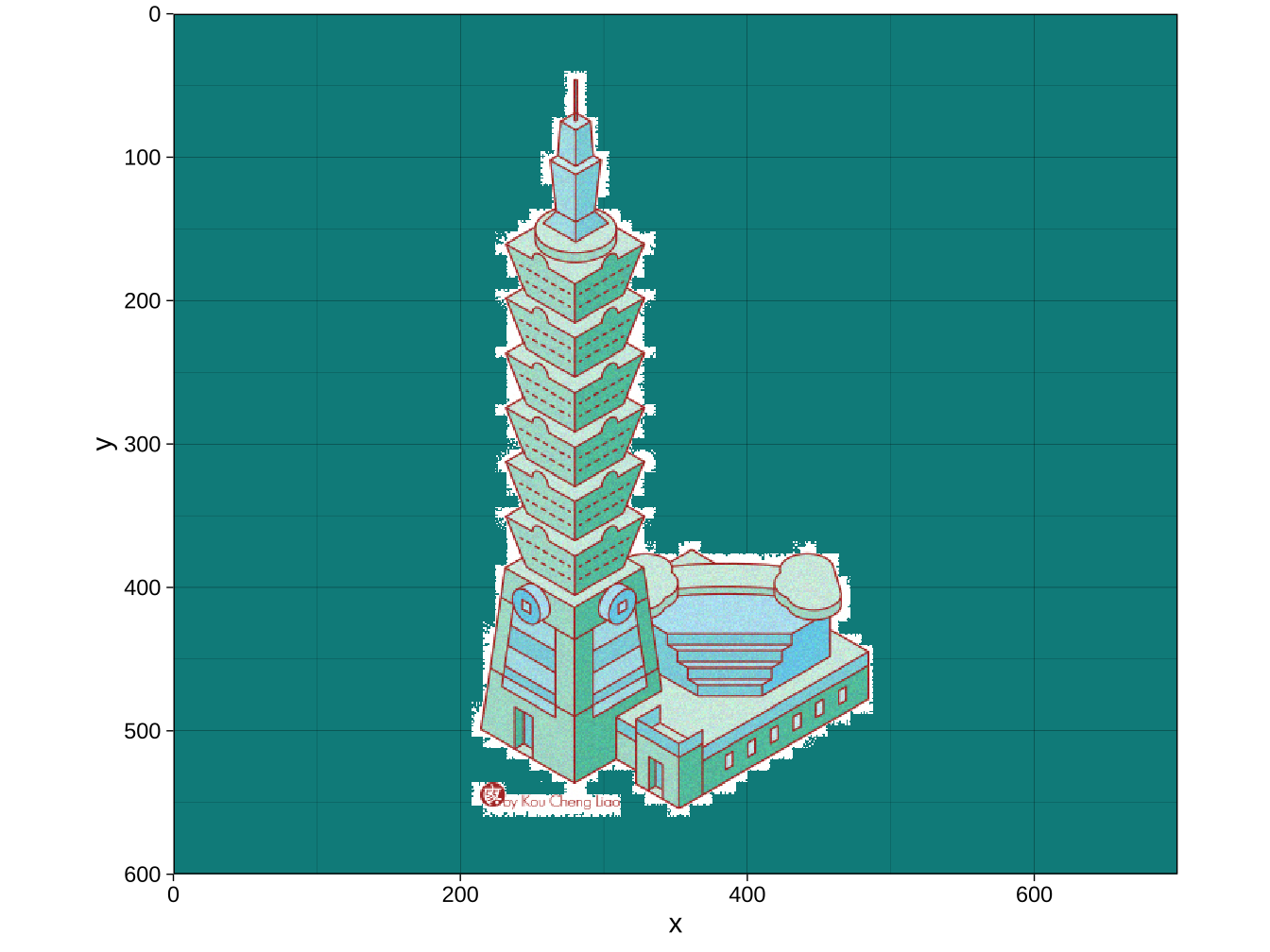

image_fill(taipei101,"transparent", point = "+100+100", fuzz=30) %>%
    image_ggplot()+list_graphs$theme_backgroundCheck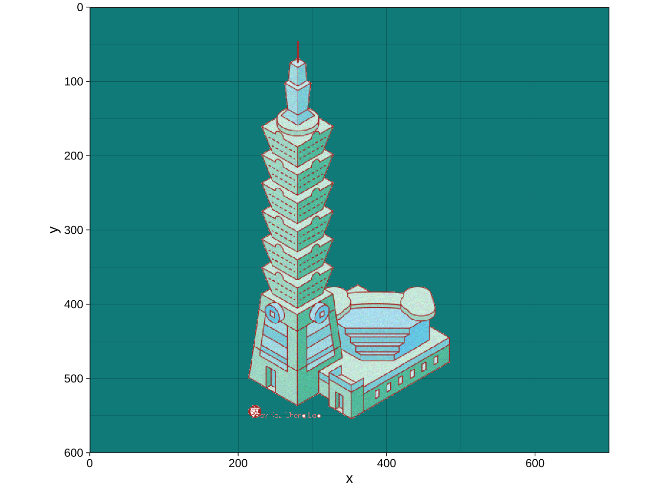

轉成raster矩陣資料

image_fill(taipei101,"transparent", point = "+100+100", fuzz=30) -> 
  taipei101transparent

taipei101transparent %>%
  as.raster() ->
  raster_taipei101

loc <- c(lon=121.5622782,lat=25.0339687) # Taipei101 經緯度
imgWidth <- 0.13 # Taipei101在圖片佔寬

list_graphs$northTW +
  annotation_raster(raster_taipei101,
                    loc[1]-imgWidth/2,loc[1]+imgWidth/2,
                    loc[2]-imgWidth/2*img_asp,loc[2]+imgWidth/2*img_asp)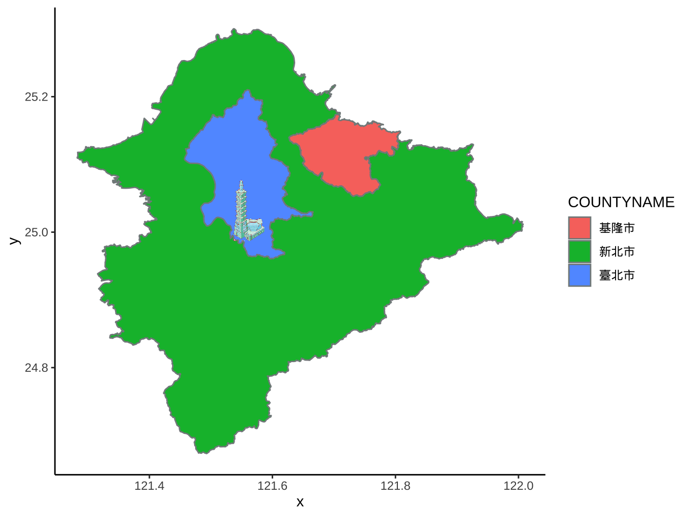

調低解析度

image_scale(taipei101transparent,"200") -> taipei101sm
taipei101sm %>% as.raster() -> raster_taipei101sm
list_graphs$northTW +
  annotation_raster(raster_taipei101sm,
                    loc[1]-imgWidth/2,loc[1]+imgWidth/2,
                    loc[2]-imgWidth/2*img_asp,loc[2]+imgWidth/2*img_asp) ->
  list_graphs$northTW2

list_graphs$northTW2

選一張過去展示作品，幫它加上

• 國立臺北大學logo:
  https://upload.wikimedia.org/wikipedia/commons/thumb/d/d3/National_Taipei_University_logo.svg/1200px-National_Taipei_University_logo.svg.png

5.2.3 QR code

library(qrcode)
qrcode_gen("https://bookdown.org/tpemartin/108-1-ntpu-datavisualization/",
           dataOutput=TRUE, plotQRcode=F) -> qr_matrix

qr_dim <- dim(qr_matrix)
qr_matrix %>%
  as.character() %>%
  str_replace_all(
    c("1"="black",
      "0"="white")
  ) -> qr_raster

dim(qr_raster) <- qr_dim

list_graphs$northTW2+
  annotation_raster(qr_raster,121.8,122.0,24.65,24.85)+
  theme_void()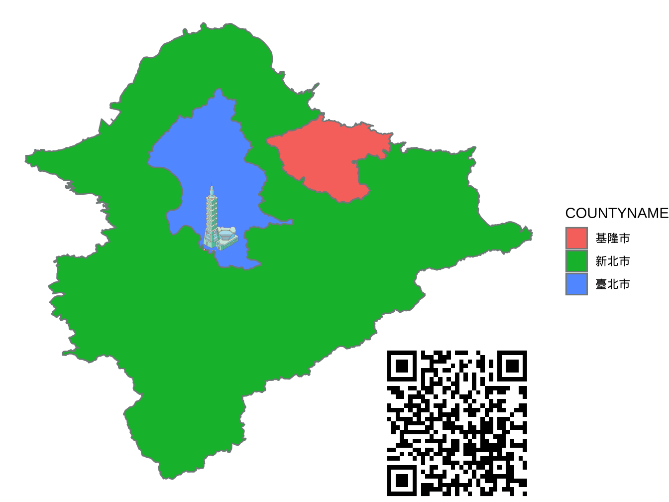

選一張過去展示作品，幫它加上

• 國立臺北大學logo

• QR code, 內容為經濟學系網址： http://www.econ.ntpu.edu.tw/econ/index.php

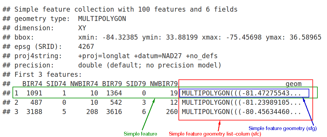
5.3 Simple features

一種地圖資訊的儲存格式，將地理區域的特徵以點、線、多邊體等簡單幾何特徴記錄。

引入simple feature處理套件

library(sf)

透過這套件我們會以下面3步驟架構sf資料：

想像構架台灣22個直轄市/縣/市

1. Simple feature geometry（sfg class）: 每個縣市由那些簡單幾何構成

2. Simple feature column（sfc class）: 將所有縣市的sfg堆疊成的column

3. Simple feature object（sf class）: 再放上所有縣市其他非地理特徵形成的完整資料物件

5.4 Coordinate Reference Systems (CRS)

包含兩部份：

• geographic coordinate reference systems: 經度、緯度，衡量規則通常為WGS84。

• projected coordinate reference systems：怎麼把球體上的地理位置投射成2維經緯平面，受投射中心點及投射方法選擇影響。

不同CRS在2維平面投出的地理形狀、兩點距離、兩點角度會有不同結果；在繪圖時需要特別聲明。

CRS設定，2選一：

• epsg碼:

• proj4string: `+proj=<投射法> A planar CRS defined by a projection, datum, and a set of parameters. In R use the PROJ.4 notation, as that can be readily interpreted without relying on software.

Definition 5.1 There are various attributes of the CRS, such as the projection, datum, and ellipsoid. Some of the options for each variable can be obtained in R with projInfo:
1. Projection: projInfo(type = “proj”) 什麼投射法
2. Datum: projInfo(type = “datum”) 什麼圖資來定義經緯線
3. Ellipsoid: projInfo(type = “ellps”) 什麼橢球體

5.5 架構sf data frame

1. simple features geometry (for each county)
   
2. simple features column (for all counties)
   
3. set simple features column as a column in a data frame

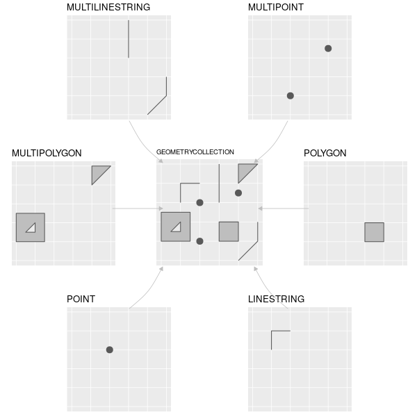
5.5.1 Geometry (sfg)

主要由以下幾種geometries構成：

POINT, LINESTRING, POLYGON, MULTIPOINT, MULTILINESTRING, MULTIPOLYGON and GEOMETRYCOLLECTION

定義函數均為st_<geometry type>(<geometry record>):

一點：st_point

point <- st_point(
  c(2,3)
)

point %>% ggplot()+geom_sf()

數個點：st_multipoint

mpoint <- st_multipoint(
    rbind(c(1,0),
        c(2,3),
        c(-1,2))
)

mpoint %>% ggplot()+geom_sf()

一條線：st_linestring

line <- st_linestring(
    rbind(c(1,0),
        c(2,3),
        c(-1,2))
)
line %>% ggplot()+geom_sf()

數條線: st_multilinestring

mline <- st_multilinestring(
  list(
    rbind(
      c(1,0),
      c(2,3),
      c(-1,3)),
    rbind(
      c(-2,3),
      c(-1,-1))
    )
  )

mline %>% ggplot()+geom_sf()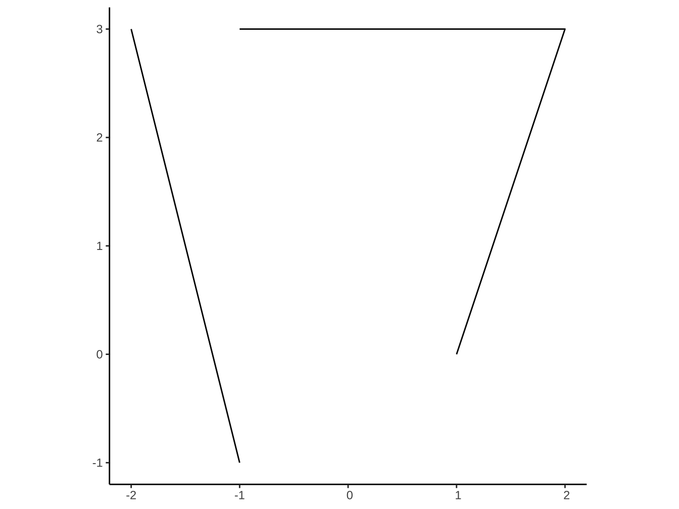

一個多邊體：st_polygon

outer <-     
  rbind( # 外圍
    c(1,5),
    c(2,1),
    c(5,1),
    c(5,5),
    c(1,5)) # 必需自行輸入起點close it

hole <-
  rbind( # 洞
    c(2,4),
    c(3,2),
    c(4,3),
    c(2,4))  # 必需自行輸入起點close it
  
poly <- st_polygon(
  list(
    outer, 
    hole
  )
) 

poly %>% ggplot()+geom_sf()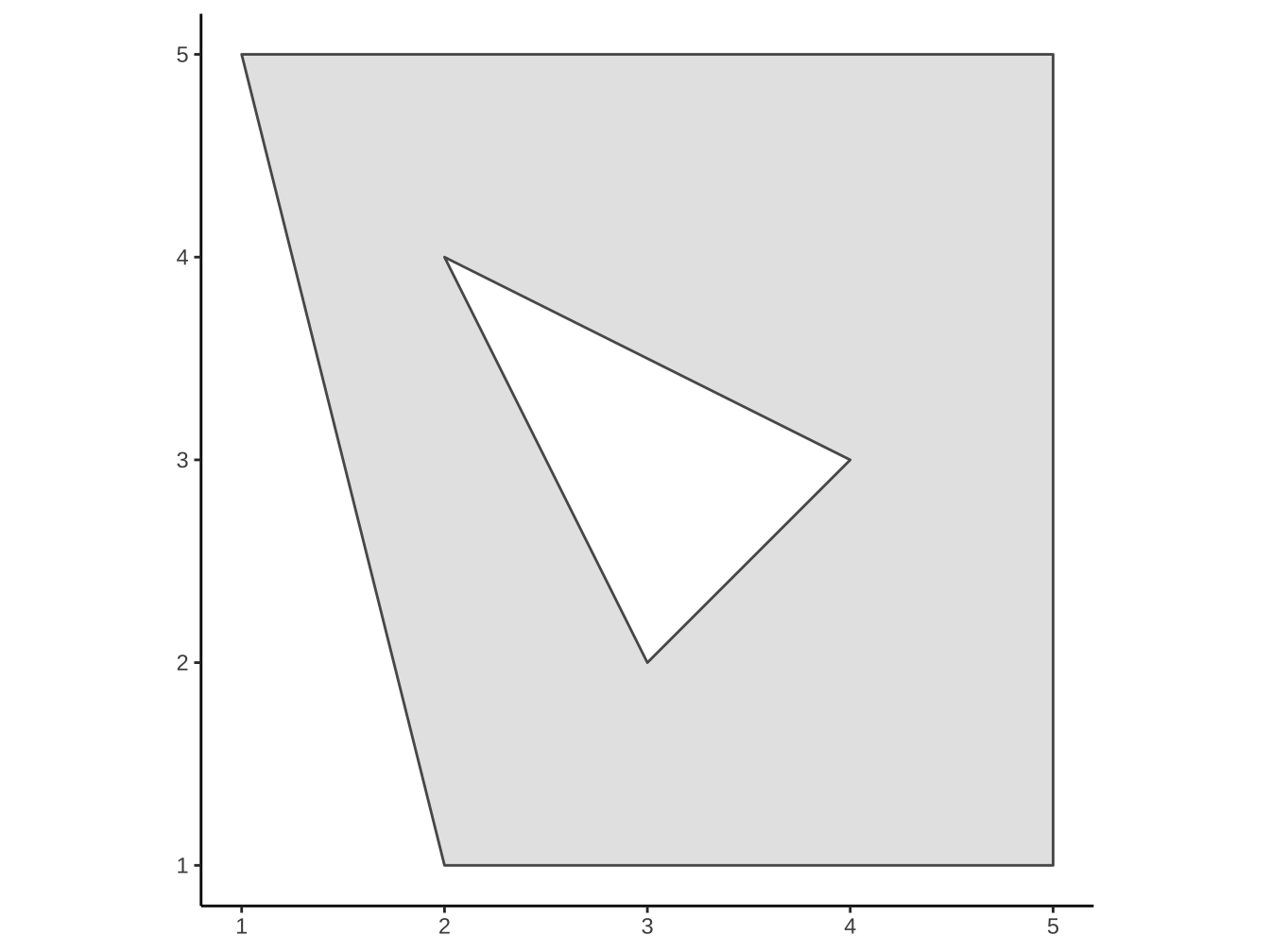

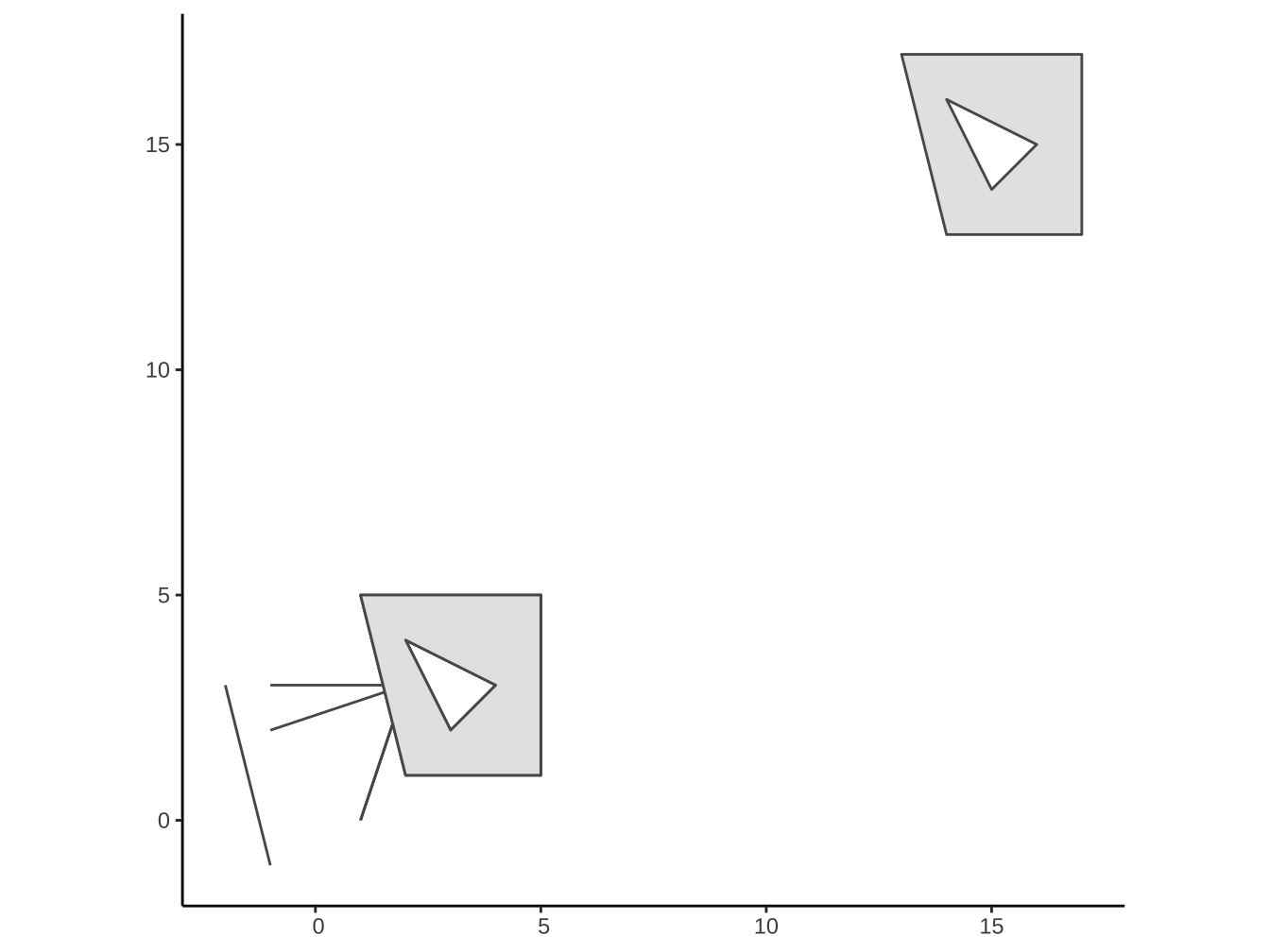
sf::st_polygon(sf)與ggplot2::geom_polygon(ggplot2)對多邊體格式定義差異：

• sf下多邊體的最後一個座標必需是第一個座標；ggplot2則不用，自動假設連回第一個 。

• sf以第一個ring（即多邊體邊界一圈）為outer ring，其餘為holes。ggplot2則需定義group及subgroup兩個變數後，才能自動判斷哪個ring為ourter，哪個ring為holes。

數個多邊體：st_multipolygon

outer2 <- outer + 12
hole2 <- hole + 12

mpoly <- st_multipolygon(
  list(
    list(
      outer,
      hole
    ),
    list(
      outer2,
      hole2
    )
  )
) 

mpoly %>% ggplot()+geom_sf()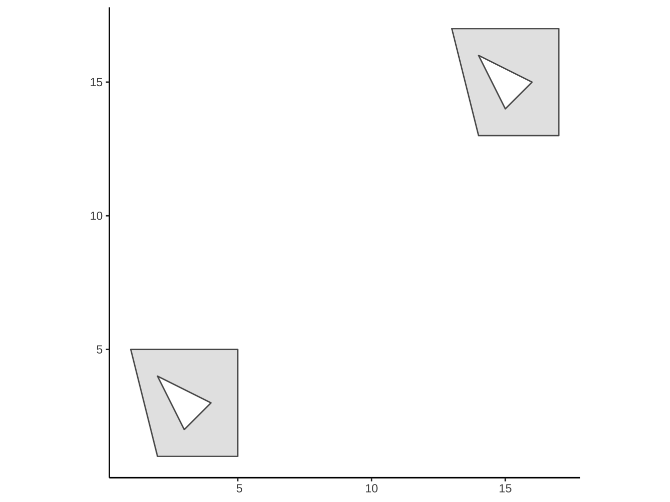

複合幾何收藏：st_geometrycollection

st_geometrycollection(
  list(
    point, mpoint,
    line, mline,
    poly, mpoly
  )
) %>% ggplot()+ geom_sf()

5.5.2 Column (sfc)

建立geometry欄位

st_sfc() to form simple features column.

sfg_county1 <- st_polygon(list(
  outer,hole
))
sfg_county2 <- st_polygon(list(
  outer2, hole2
))

sfc_county12column <- st_sfc(sfg_county1,sfg_county2)

sfc_county12column %>% ggplot+geom_sf()

設定CRS

架構sfc後，最好也順便設定CRS:

sfc_county12column %>%
  st_set_crs(4326) -> # EPSG: 4326
  sfc_county12column

5.5.3 與data frame合併 (sf)

形成sf object: a data frame with a geometry column

Given a data frame, say df, we can attach a geometry column (sfc), say geo_column, through:

st_set_geometry(df,geo_column)

df_county12 <- data.frame(
  name=c("county1","county2"),
  population=c(100,107)
)

df_county12 %>%
  st_set_geometry(sfc_county12column) -> df_county12

df_county12 %>% names

[1] “name” “population” “geometry”

5.5.4 儲存成shp檔

dir.create("county12")
write_sf(df_county12,"county12/county12.shp")

當然如果只是個人要用，或確信對方也使用R，你也可以存成Rda檔。

save(df_county12,file="df_county12.Rda")

之後再：

load("df_county12.Rda")

資料來源：政府資料開放平台（https://data.gov.tw/dataset/73233）
執行取得sf_mrt_tpe

load(url("https://www.dropbox.com/s/uvco1te2kbs6o01/MRT_Taipei.Rda?dl=1"))

其中代號’O’為「中和新蘆線」、’BL’為「板南線」，只取出此兩線，並形成一個sf data frame含有以下欄位：

• 路線名稱

• geometry: 代表各路線的「點、線」圖。

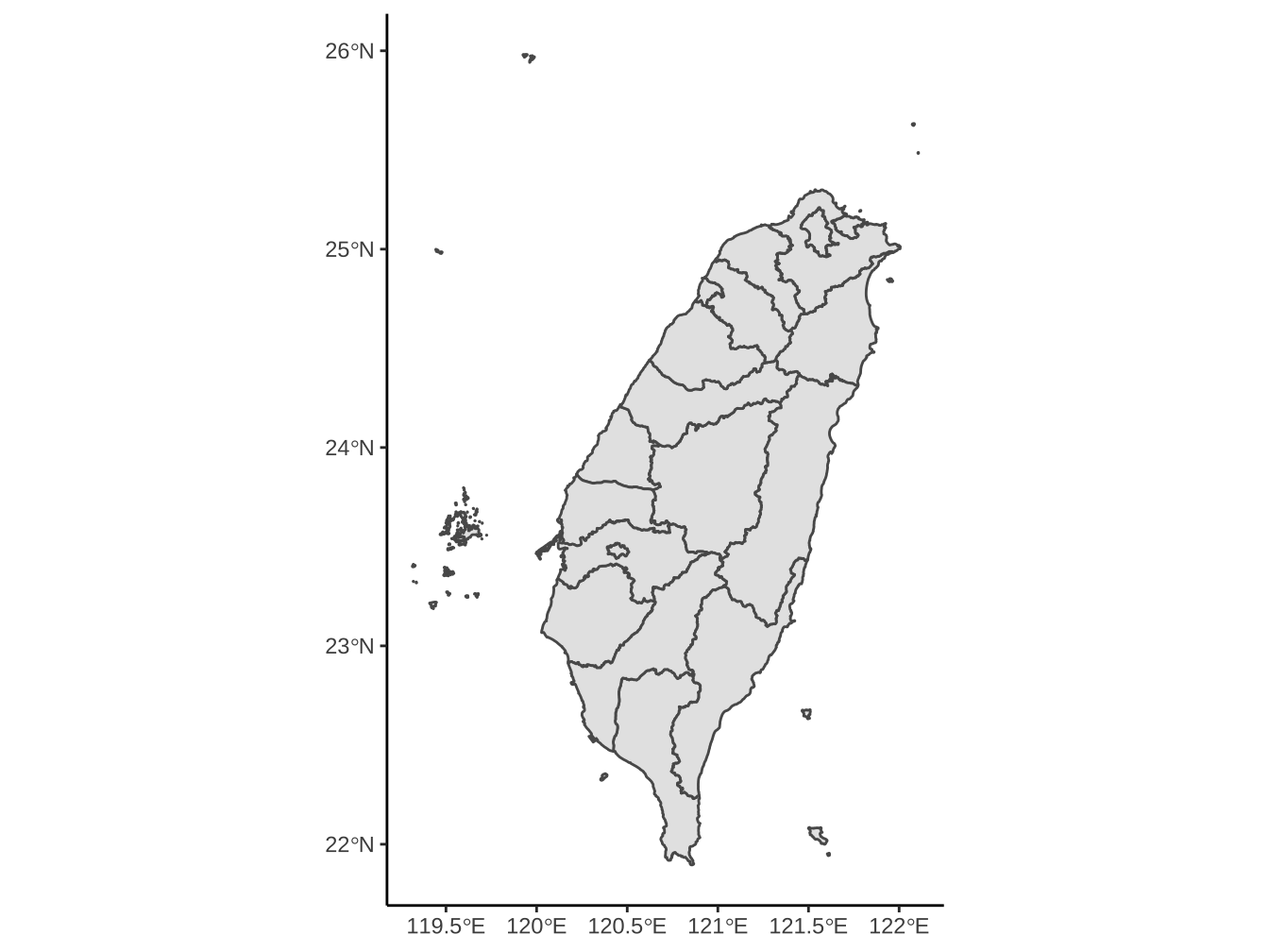
5.6 讀入shp檔

shp檔其實是由數個檔形成的向量地理圖資，包含：.shp, .shx, .dbf （前三個必需要有）及 .prj等一系列「相同名稱」、「不同副檔名」組成的地理資訊。

sf::read_sf(".shp檔位置")

sf_county12=read_sf("county12/county12.shp")

由 https://data.gov.tw/dataset/7442 引入台灣直轄市、縣市界線圖資存在名為sf_taiwan的物件。

5.7 常見圖資運算

5.7.1 CRS轉換: st_transform()

# 取出spData套件附的world data
data(world,package="spData")
class(world) # 已是sf object

[1] “sf” “tbl_df” “tbl” “data.frame”

# 目前CRS
world %>% st_crs 

Coordinate Reference System: EPSG: 4326 proj4string: “+proj=longlat +datum=WGS84 +no_defs”

world %>% st_geometry() %>%
  ggplot()+geom_sf()

更換CRS

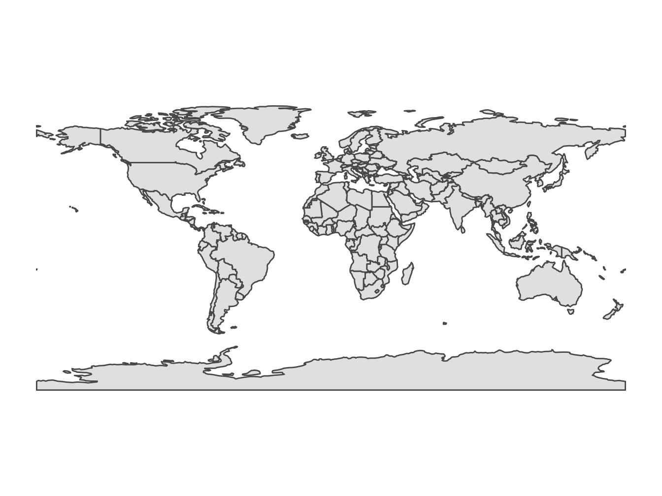
world %>% 
  st_transform(crs="+proj=laea +y_0=0 +lon_0=155 +lat_0=-90 +ellps=WGS84 +no_defs") -> world_proj
  
world_proj %>%
  ggplot()+geom_sf()

5.7.2 找中心點： st_centroid()

• 找polygon中心點

• 形成新的sf object，有相同data frame但geometry column只是中心點的point geometry.

• 如果一筆feature資料有多個中心點，可以設定：
  st_centroid(..., of_largest_polygon = T)

load(url("https://www.dropbox.com/s/elnvocol0nnkcc9/sf_northTaiwan.Rda?dl=1"))

sf_northTaiwan %>%
  st_centroid(of_largest_polygon = T) ->
  sf_centroid_northTaiwan

sf_centroid_northTaiwan

Simple feature collection with 3 features and 4 fields geometry type: POINT dimension: XY bbox: xmin: 121.6 ymin: 24.99 xmax: 121.7 ymax: 25.12 epsg (SRID): 3824 proj4string: +proj=longlat +ellps=GRS80 +towgs84=0,0,0,0,0,0,0 +no_defs # A tibble: 3 x 5 COUNTYID COUNTYCODE COUNTYNAME COUNTYENG *
1 C 10017 基隆市 Keelung … 2 A 63000 臺北市 Taipei C… 3 F 65000 新北市 New Taip… # … with 1 more variable: geometry <POINT [°]>

5.7.3 輸出座標: st_coordinates()

找中心點有時是為了做圖加上新的geom_point layer，還會再進行geom_point layer data frame架構：

sf_centroid_northTaiwan %>%
  st_coordinates() -> coord_centroid_northTaiwan # 取出座標

coord_centroid_northTaiwan

  X     Y

1 121.7 25.12 2 121.6 25.08 3 121.6 24.99

sf_northTaiwan$x_centroid <- coord_centroid_northTaiwan[,"X"]
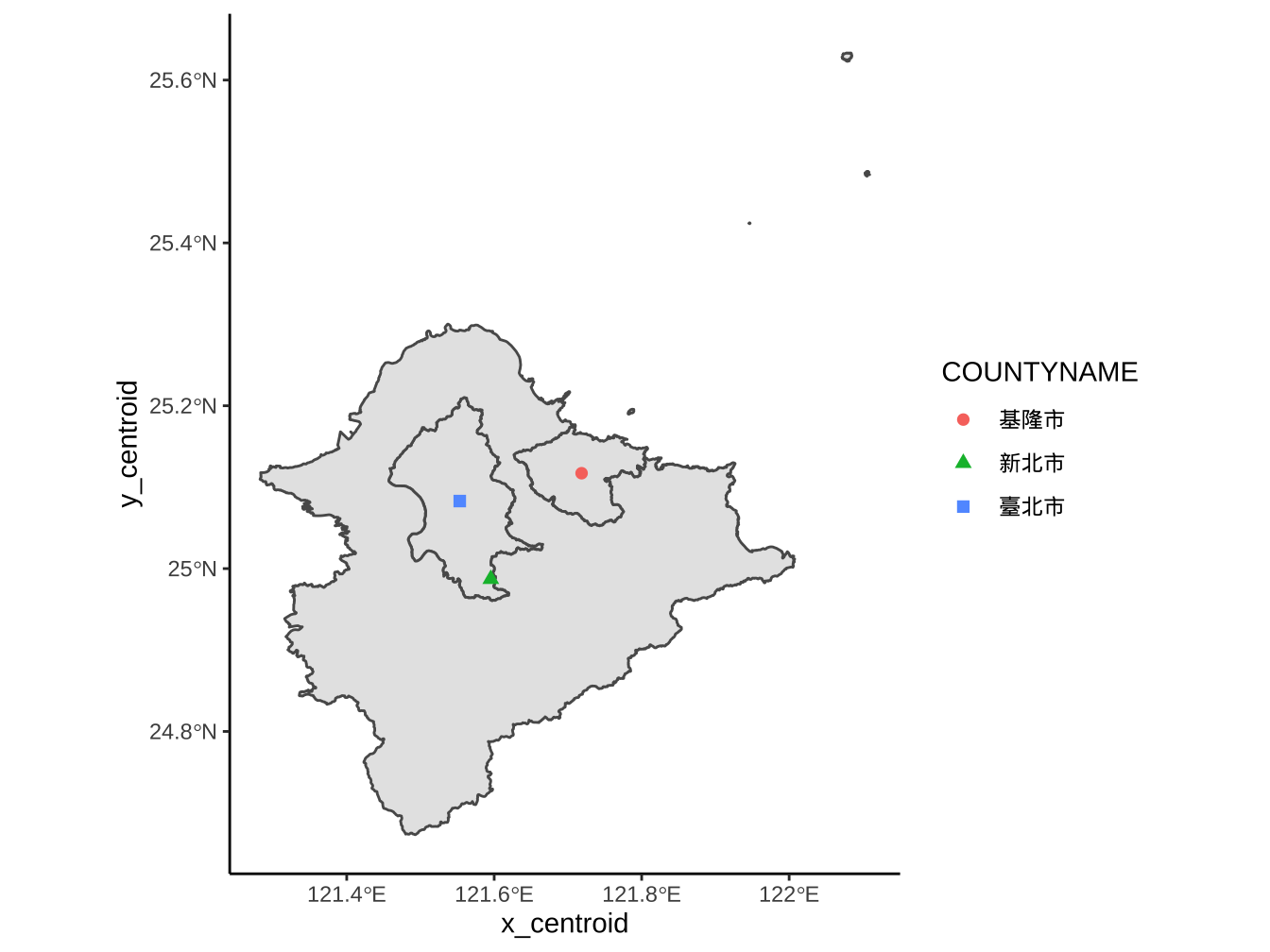
sf_northTaiwan$y_centroid <- coord_centroid_northTaiwan[,"Y"]

sf_northTaiwan %>%
  ggplot()+
  geom_sf()+
  geom_point(
    aes(
      x=x_centroid,y=y_centroid, 
      shape=COUNTYNAME, color=COUNTYNAME
    ), size=2
  )

5.7.4 切出部份範圍: st_crop()

sf_northTaiwan %>%
  ggplot()+geom_sf()

sf_northTaiwan %>%
  st_crop(xmin=121.2,xmax=122,ymin=24.6,ymax=25.3) %>%
  ggplot()+geom_sf()

5.7.5 幾何簡化: rmapshaper::ms_simplify()

接續5.6的台灣圖資：

sf_taiwan %>%
  rmapshaper::ms_simplify() -> sf_taiwan_simplify

sf_taiwan_simplify %>%
  st_crop(
    xmin=119, xmax=123,
    ymin=21, ymax=26
  ) %>%
  ggplot()+geom_sf()

5.7.6 st_cast

5.7.7 更多其他操作

• https://r-spatial.github.io/sf/index.html

• geometrical operations:
  https://r-spatial.github.io/sf/articles/sf3.html#geometrical-operations

• cheatsheet:
  https://github.com/rstudio/cheatsheets/blob/master/sf.pdf

5.8 ggplot地圖繪製

• https://ggplot2.tidyverse.org/reference/ggsf.html

5.8.1 繪製goemetry: geom_sf()

world %>%
  ggplot()+geom_sf()

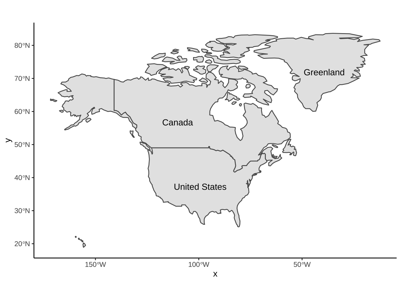
5.8.2 加文字: geom_sf_text(), geom_sf_label()

geometry+text

world %>% 
  filter(
    subregion=="Northern America"
  ) %>% 
  ggplot()+geom_sf()+
  geom_sf_text(
    aes(label=name_long)
  )

5.8.3 設座標系統: coord_sf()

• 只對圖面上geom_sf類圖層有作用。

load(url("https://www.dropbox.com/s/1jwm27dhh4874ch/sf_tpe_mrt.Rda?dl=1"))

sf_taipei %>% st_crs

Coordinate Reference System: EPSG: 3824 proj4string: “+proj=longlat +ellps=GRS80 +towgs84=0,0,0,0,0,0,0 +no_defs”

sf_mrt_tpe_BL %>% st_crs

Coordinate Reference System: EPSG: 3826 proj4string: “+proj=tmerc +lat_0=0 +lon_0=121 +k=0.9999 +x_0=250000 +y_0=0 +ellps=GRS80 +towgs84=0,0,0,0,0,0,0 +units=m +no_defs”

不同CRS畫在一起時，ggplot會以第一層的CRS為主，主動改其他不同的CRS：

sf_taipei %>% # 第一層是sf_taipei, 以它的CRS為主
  ggplot()+
  geom_sf(
    aes(fill=COUNTYNAME)
  )+
  geom_sf(
    data=sf_mrt_tpe_BL
  ) -> tpe_mrt_map1 
tpe_mrt_map1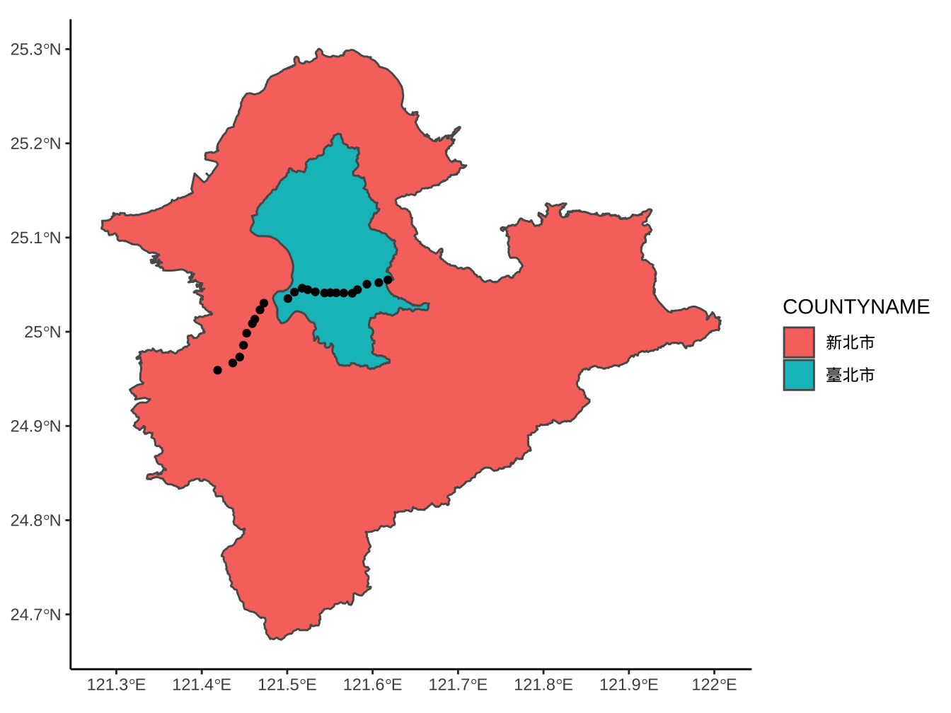

sf_mrt_tpe_BL %>% # 第一層是sf_mrt_tpe_BL, 以它的CRS為主
  ggplot()+
  geom_sf(
    data = sf_taipei,
    aes(fill=COUNTYNAME)
  )+
  geom_sf() -> tpe_mrt_map2
tpe_mrt_map2

使用coord_sf(xlim=...,ylim=...)限縮範圍：

tpe_mrt_map1 + # 以sf_taipei CRS為主
  coord_sf(
    xlim=c(121.35,121.8),
    ylim=c(24.9,25.1)
    )+
  labs(title="以sf_taipei CRS為主去限縮") -> tpe_mrt_map1_limit

tpe_mrt_map2 + # 以sf_mrt_tpe_BL CRS為主
  coord_sf(
    xlim=c(121.35,121.8),
    ylim=c(24.9,25.1)
    )+
  labs(title="以sf_mrt_tpe_BL CRS為主去限縮") -> tpe_mrt_map2_limit

以sf_mrt_tpe_BL CRS為主時，圖會不見：

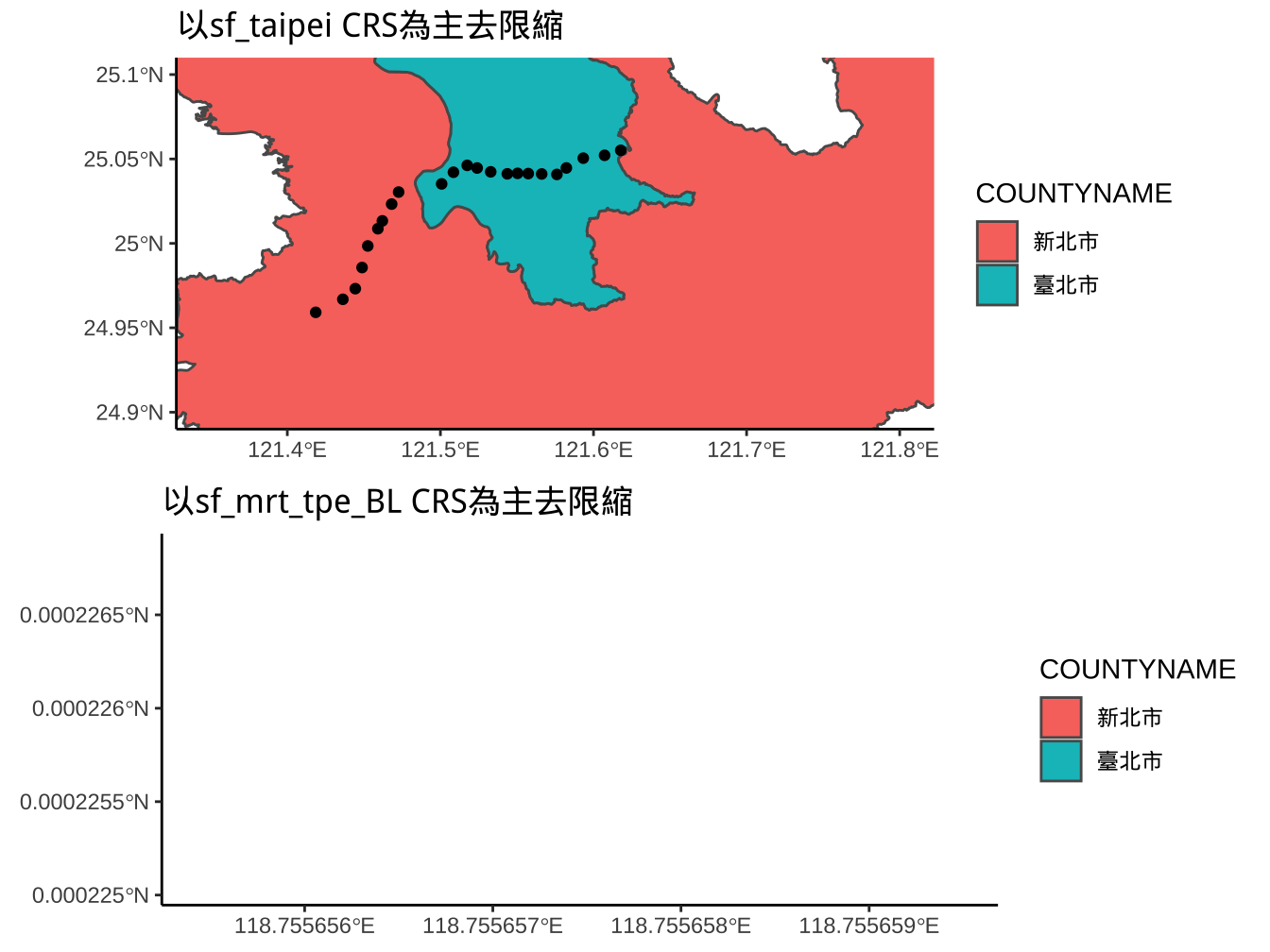
geom_sf圖面的座標是我們label後的結果，即如同scale_x_continuous(limits=..., breaks=..., labels=...)中的label，而xlim和ylim是在控制真實資料limits的範圍。

sf_mrt_tpe_BL %>% st_bbox()

xmin ymin xmax ymax 292263 2761319 312333 2772024

sf_taipei %>% st_bbox()

xmin ymin xmax ymax 121.28 24.67 122.01 25.30

方法一：所有sf有相同CRS

sf_mrt_tpe_BL %>%
  st_transform(st_crs(sf_taipei)) %>%
  ggplot()+
  geom_sf(
    data = sf_taipei,
    aes(fill=COUNTYNAME)
  )+
  geom_sf() -> tpe_mrt_map2_2

tpe_mrt_map2_2 + # sf_mrt_tpe_BL CRS改為sf_taipei CRS
  coord_sf(
    xlim=c(121.35,121.8),
    ylim=c(24.9,25.1)
    )

5.8.3.1 方法二：在coord_sf()內調整

tpe_mrt_map2 + # 以sf_mrt_tpe_BL CRS為主
  coord_sf(
    xlim=c(121.35,121.8),
    ylim=c(24.9,25.1),
    crs=st_crs(sf_taipei) # 要求所有sf轉成sf_taipei CRS
    )

方法二有一個缺點，若layer有非sf圖層，在此法下，其他layers的圖層可能會消失。

5.9 練習：捷運車站

資料來源：政府資料開放平台（https://data.gov.tw/dataset/73233）
執行取得sf_mrtStops_tpe

load(url("https://www.dropbox.com/s/uvco1te2kbs6o01/MRT_Taipei.Rda?dl=1"))

5.9.1 CRS

• 取出地圖CRS。

sf_mrtStops_tpe %>%
  st_crs() -> sf_mrtStops_tpe_crs
sf_mrtStops_tpe_crs

Coordinate Reference System: EPSG: 3826 proj4string: “+proj=tmerc +lat_0=0 +lon_0=121 +k=0.9999 +x_0=250000 +y_0=0 +ellps=GRS80 +towgs84=0,0,0,0,0,0,0 +units=m +no_defs”

5.9.2 取出單線站點

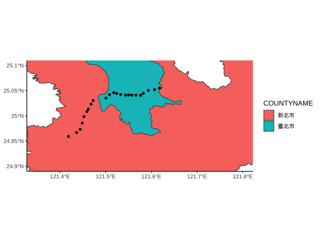
• 取出藍線（BL）畫出它的站點。

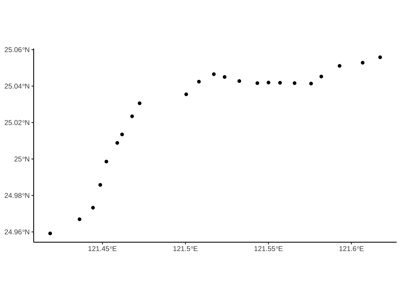
• 使用sf::st_coordinates()取出這些點的座標值。這些座標值是我們習慣的經、緯度嗎？

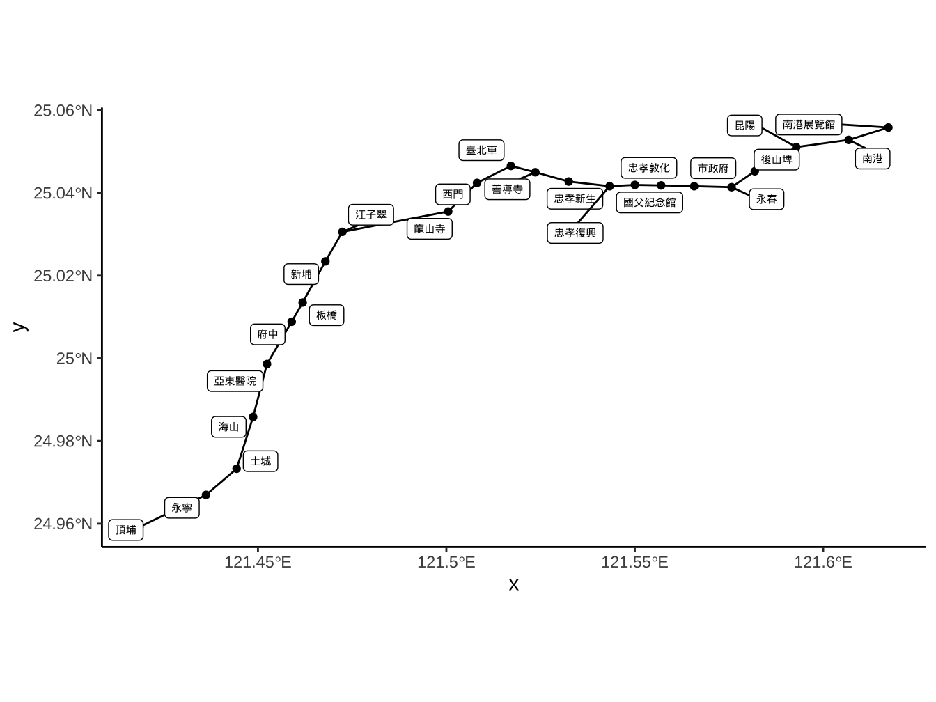
5.9.3 站點連成路線

• 將站點連成線

作法一：使用geom_path()

mrt_BL0 +
  geom_path(
    data=sf_mrtStops_tpe_BL %>% 
            mutate(
              站號=str_extract(經過路線,"(?<=(BL))[:digit:]+")
            ) %>%
            arrange(站號),
    aes(x=x,y=y)
  ) -> mrt_BL1

mrt_BL1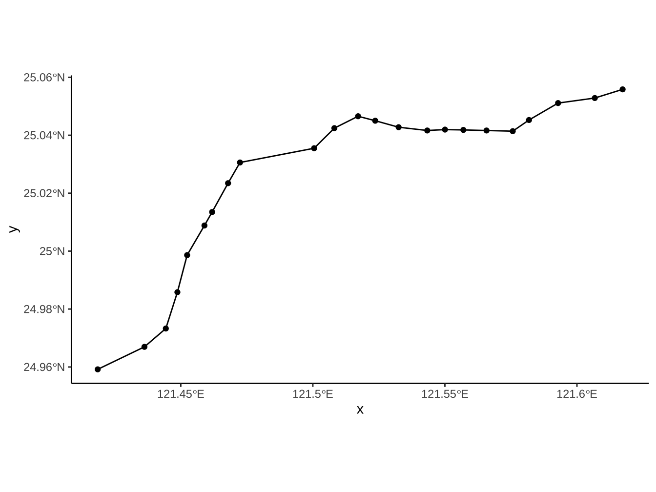

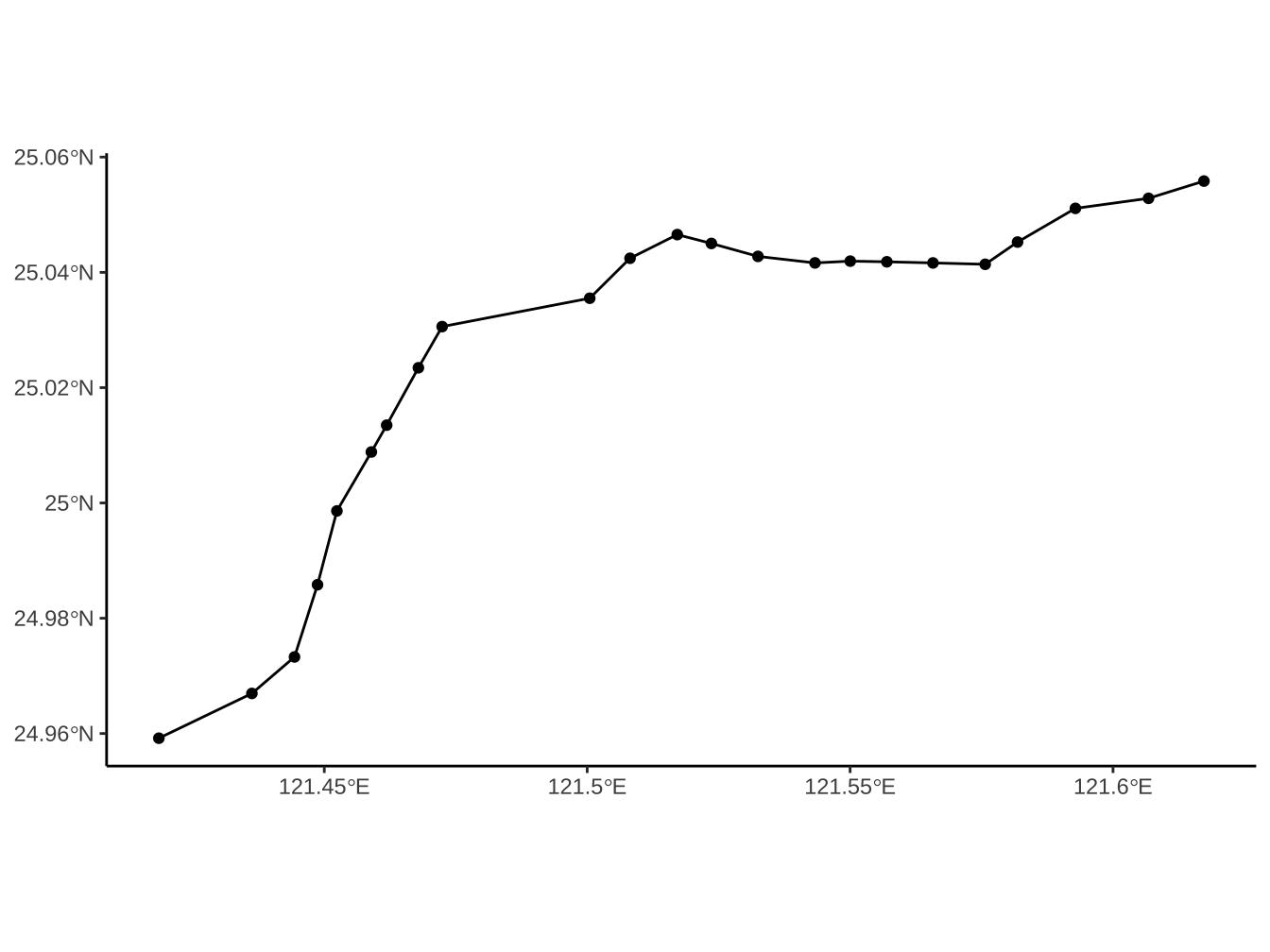
作法二：使用st_coordinates %>% st_linestring %>% sf_sfc

sf_mrtStops_tpe_BL %>% 
  mutate(
    站號=str_extract(經過路線,"(?<=(BL))[:digit:]+")
  ) %>%
  arrange(站號)  %>%
  st_geometry() %>%
  st_coordinates() %>% # matrix of coordinates
  st_linestring() %>%
  st_sfc() -> sfc_mrtline_BL

sfc物件可以進行CRS設定

sf_mrtStops_tpe %>% 
  st_crs -> crs0

sfc_mrtline_BL %>%
  st_set_crs(crs0) -> sfc_mrtline_BL

在原本的站點圖再加上路線：

mrt_BL0 +
  geom_sf(
    data=sfc_mrtline_BL
  )

5.9.4 標站名

• 標上站名

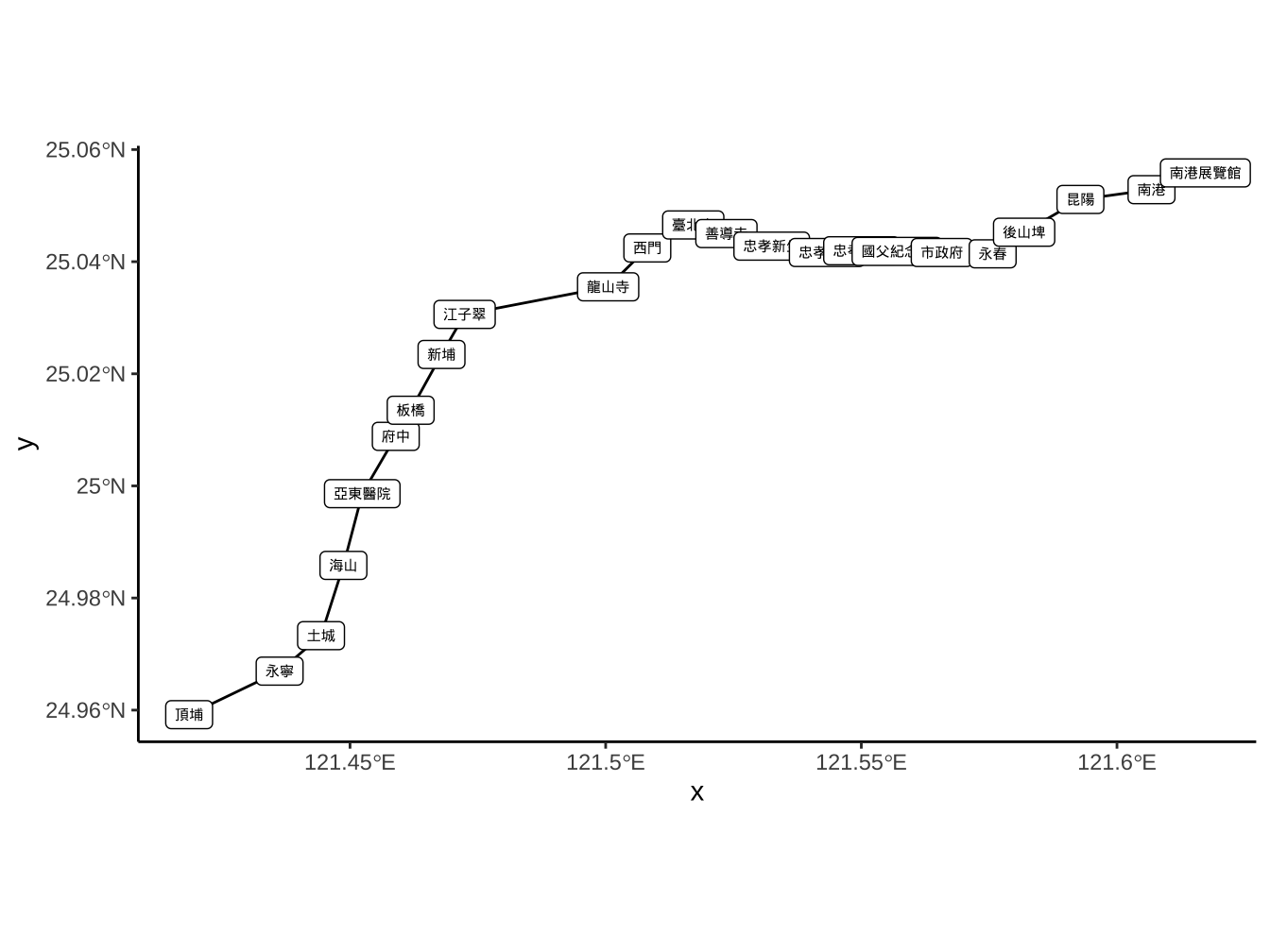
ggrepel套件特別為geom_text及geom_label設計了不重疊、自動閃避的geom_text_repel及geom_label_repel元素。

• 放上大台北地圖(可不放站名)

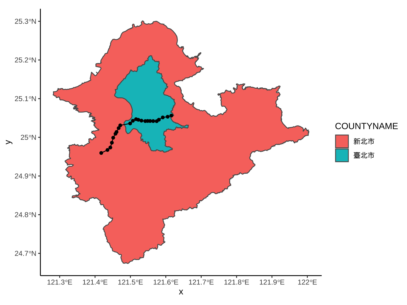
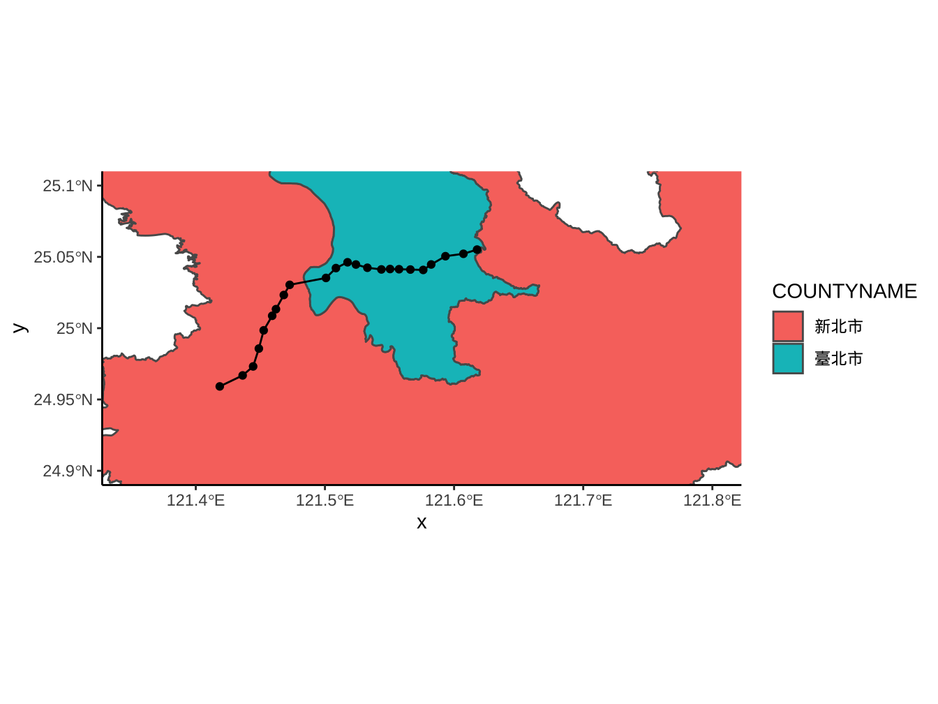
• 使用ggplot2::coord_sf() layer或sf::st_crop()將圖面限縮在東經121.35到121.8度，及北緯24.9到25.1度間。

5.10 其他相關圖資套件

5.10.1 osmdata

• open street map: https://www.openstreetmap.org/

• https://ropensci.github.io/osmdata/

• https://ropensci.github.io/osmdata/articles/index.html

library(osmdata)

5.10.1.1 網頁下載.osm

download.file("https://www.dropbox.com/s/wisgdb03j01js1r/map.osm?dl=1",
              destfile = "map.osm")
st_layers("map.osm")

st_read("map.osm",layer="lines") -> sf_ntpu_lines

Reading layer lines' from data source/Users/martin/Desktop/GitHub/Courses/course-data-visualization/108-1/map.osm’ using driver `OSM’ Simple feature collection with 218 features and 9 fields geometry type: LINESTRING dimension: XY bbox: xmin: 121.3 ymin: 24.93 xmax: 121.4 ymax: 24.97 epsg (SRID): 4326 proj4string: +proj=longlat +datum=WGS84 +no_defs

st_read("map.osm",layer="points") -> sf_ntpu_points

Reading layer points' from data source/Users/martin/Desktop/GitHub/Courses/course-data-visualization/108-1/map.osm’ using driver `OSM’ Simple feature collection with 369 features and 10 fields geometry type: POINT dimension: XY bbox: xmin: 121.3 ymin: 24.93 xmax: 121.4 ymax: 24.96 epsg (SRID): 4326 proj4string: +proj=longlat +datum=WGS84 +no_defs

st_read("map.osm",layer="multipolygons") -> sf_ntpu_multipolygons

Reading layer multipolygons' from data source/Users/martin/Desktop/GitHub/Courses/course-data-visualization/108-1/map.osm’ using driver `OSM’ Simple feature collection with 258 features and 25 fields geometry type: MULTIPOLYGON dimension: XY bbox: xmin: 121.4 ymin: 24.94 xmax: 121.4 ymax: 24.95 epsg (SRID): 4326 proj4string: +proj=longlat +datum=WGS84 +no_defs

sf_ntpu_points %>% View("points")
sf_ntpu_lines %>% View("lines")
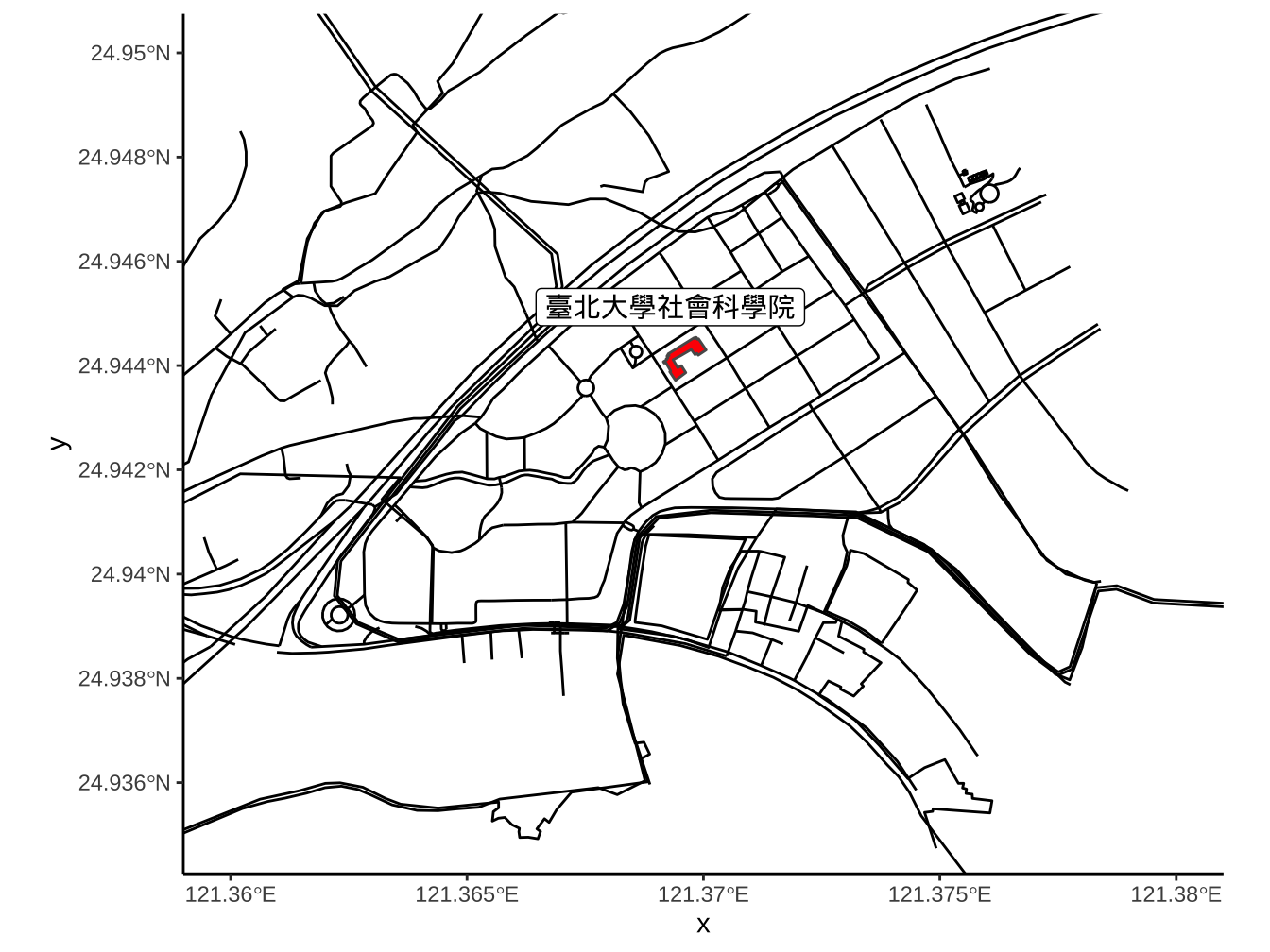
sf_ntpu_multipolygons %>% View("multipolys")

sf_ntpu_lines %>%
  ggplot()+geom_sf()+
  geom_sf(
    data=sf_ntpu_multipolygons %>%
      filter(
        name=="臺北大學社會科學院"
      ),
    fill="red"
  )+
  geom_sf_label(
    data=sf_ntpu_multipolygons %>%
      filter(
        name=="臺北大學社會科學院"
      ),
    aes(label=name), nudge_y = 0.001
    )+
  coord_sf(
    xlim=c(121.36,121.38),
    ylim=c(24.935,24.95)
  )

5.10.1.2 Overpass query

• bbox (bounding box): c(xmin,ymin,xmax,ymax) (由左側逆時針數)

• osm feature:

  • key-value查詢: https://wiki.openstreetmap.org/wiki/Map_Features

bbox

library(osmdata)
# open pass query with bounding box
bbox_taipei <- opq(
  bbox = c(121.4616,25.1050,121.6058,24.9894) 
) 

add feature

捷運線

railway:subway

bbox_taipei %>% 
  add_osm_feature(
    key="railway", value="subway"
  ) %>%
  osmdata_sf() -> map_taipei_subway

map_taipei_subway

原始資料

map_taipei_subway$osm_lines %>% View

同路線會散佈在分開記錄的linestring裡，要先合併。

map_taipei_subway$osm_lines %>%
  mutate(
    length=st_length(geometry),
    shortname=str_replace(name,"捷運","") %>%
      str_extract("[:graph:]+(?=線)")
  ) -> sf_tpe_mrt

範例：將各個板南線片段連起來（使用st_union()）

sf_tpe_mrt %>%
  filter(
    shortname=="板南"
  ) %>%
  st_geometry() -> sfc_BL
sfc_BL %>% st_union() %>%
  ggplot()+geom_sf()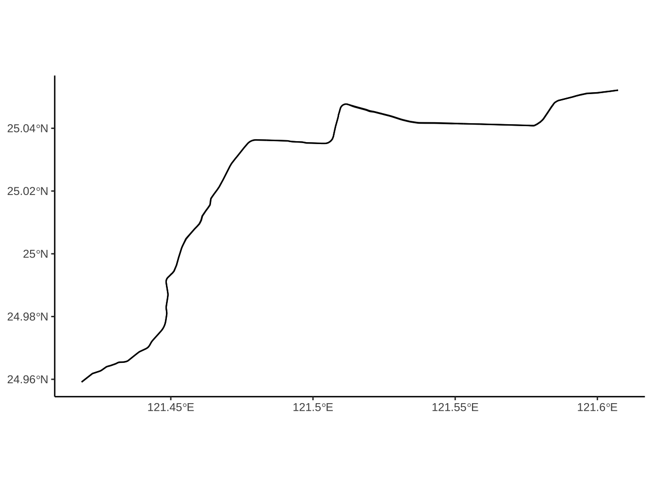

將各路線片段資料整合在一起，並去除NA

sf_tpe_mrt %>%
group_by(
    shortname
  ) %>%
  summarise(
    geometry=st_union(geometry)
  ) %>%
  ungroup() %>%
  na.omit() -> sf_tpe_mrt


sf_tpe_mrt %>%
  ggplot()+geom_sf(
    aes(color=shortname, fill=shortname), size=1
  ) +
  geom_sf_text(
    aes(label=shortname)
  )+
  labs(title="台北捷運路線圖")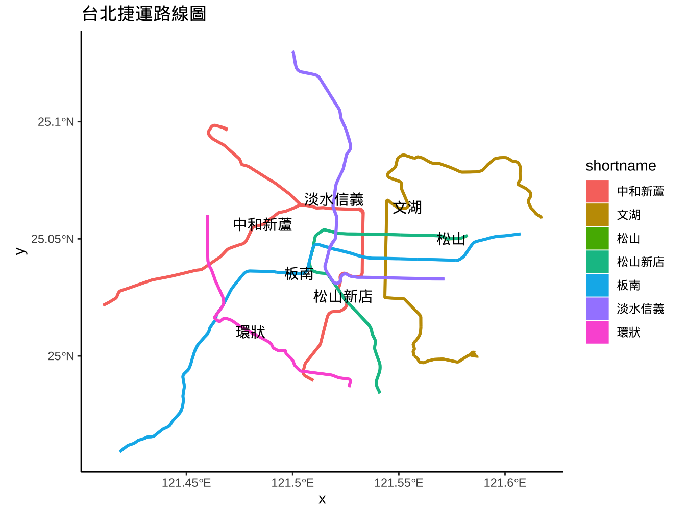

結合台北捷運站圖資，點上捷運站。

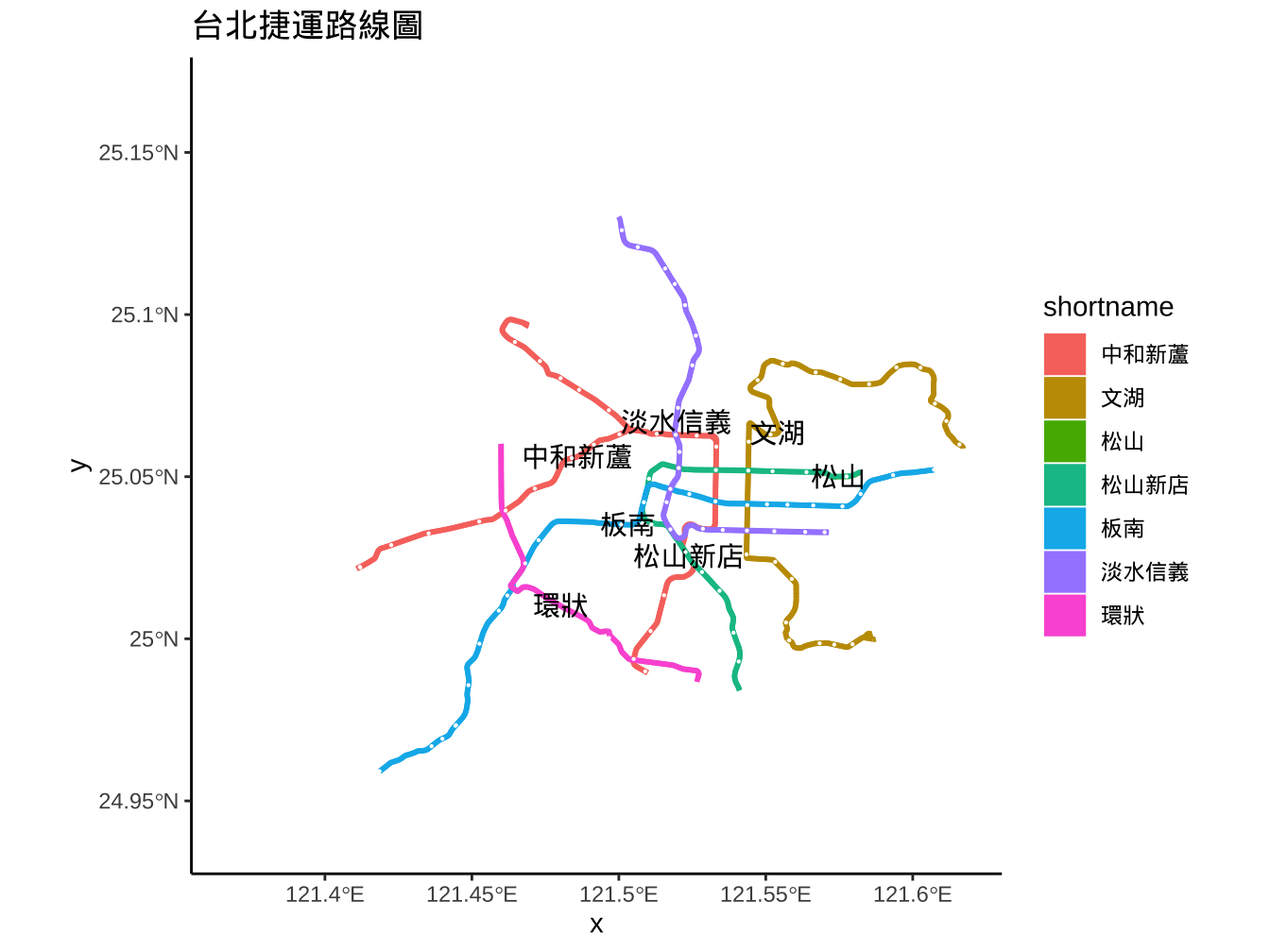
行政區

admin_level: 5

bbox_taipei %>%
  add_osm_feature(
    key="admin_level", value="5"
  ) %>%
  osmdata_sf() -> map_taipei_boundary

map_taipei_boundary  

map_taipei_boundary$osm_multipolygons -> map_taipei

osm資料對於每一個feature的geometry元素皆有命名，且此名稱是所有geometry feature代碼的串接，因此名稱會太長，超過R內定可容忍長度，而產生如下Error:

map_taipei %>%
  ggplot()+
  geom_sf()

Error in do.call(rbind, x) : variable names are limited to 10000 bytes

下面程式碼會將命稱改以簡單數字命名：

map_taipei %>%
  st_geometry() -> sfc_map_taipei
for(i in seq_along(sfc_map_taipei)){
  names(sfc_map_taipei[[i]][[1]]) <-
    1:length(names(sfc_map_taipei[[i]][[1]]))
}

map_taipei %>%
  st_set_geometry(
    sfc_map_taipei
  ) -> map_taipei2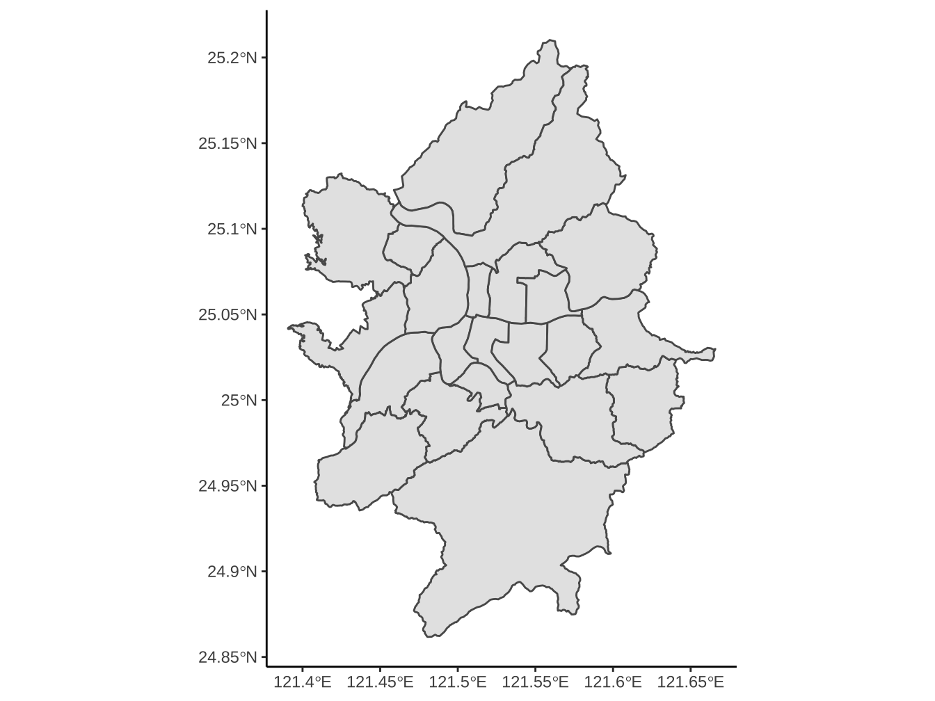

map_taipei2 %>%
  ggplot()+
  geom_sf()

osm_geom_rename

寫成函數方便未來反覆使用

osm_geom_rename <- function(sf_object){
  sf_object %>%
    st_geometry() -> sfc_sf_object
  for(i in seq_along(sfc_sf_object)){
    names(sfc_sf_object[[i]][[1]]) <-
      1:length(names(sfc_sf_object[[i]][[1]]))
  }
  
  sf_object %>%
    st_set_geometry(
      sfc_sf_object
    ) -> sf_object2
  return(sf_object2)
}

老師將上述函數放在以下網址，同學也可以在setup裡增加以下指令：

source("https://www.dropbox.com/s/8ndtvzqbdb4cb93/data_visulaization_pk.R?dl=1")

這樣osm_geom_rename()就進來了。

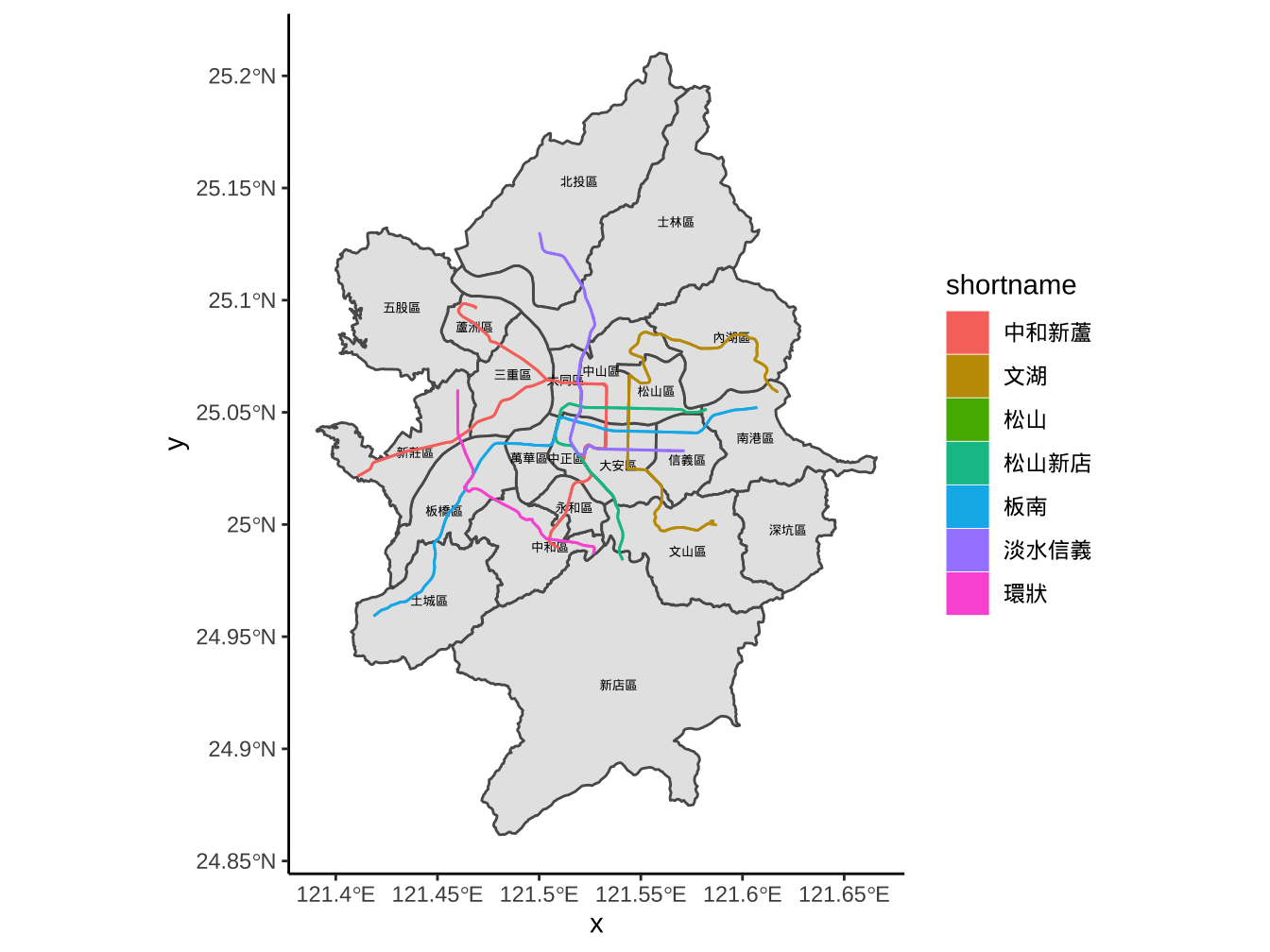
map_taipei %>%
  osm_geom_rename() %>%
  ggplot()+
  geom_sf()+
  geom_sf_text(
    aes(label=name), size=5/.pt
  )+
  geom_sf(
    data=sf_tpe_mrt, 
    aes(color=shortname, fill=shortname),
    size=0.5
  )

5.10.2 ggmap

An R package that makes it easy to retrieve raster map tiles from popular online mapping services like Google Maps and Stamen Maps and plot them using the ggplot2 framework.

• https://github.com/dkahle/ggmap

• 使用Google maps service必需先至Google Maps Platform註冊（需要設帳單資訊）才能使用。

devtools::install_github("dkahle/ggmap")

5.10.3 RQGIS

• http://www.qgistutorials.com/zh_TW/index.html

  • http://www.qgistutorials.com/zh_TW/docs/downloading_osm_data.html

  • Download open street map data: https://www.qgistutorials.com/en/docs/3/downloading_osm_data.html

5.11 其他圖資格式

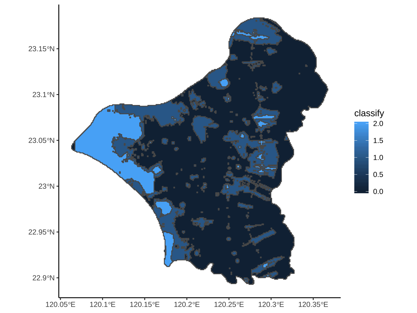
5.11.1 Raster

5.11.2 GeoJSON

library(geojsonsf)
geojson_sf("https://data.tainan.gov.tw/dataset/175c9778-62d5-4bb4-b19a-1d8171632ce4/resource/1ff9b2d6-9764-45b5-940d-c72073b6b469/download/liquefaction.json") ->
  sf_tainan_soil

sf_tainan_soil %>% #View
  # rmapshaper::ms_simplify() %>%
  ggplot()+
  geom_sf(
    aes(fill=classify)
  )

5.12 Reference

• Geocomputation with R: https://geocompr.robinlovelace.net/

• Simple feature vignettes: https://cran.r-project.org/web/packages/sf/index.html

• https://docs.qgis.org/testing/en/docs/gentle_gis_introduction/coordinate_reference_systems.html

• https://jakevdp.github.io/PythonDataScienceHandbook/04.13-geographic-data-with-basemap.html

• https://www.nceas.ucsb.edu/~frazier/RSpatialGuides/OverviewCoordinateReferenceSystems.pdf

• http://www.qgistutorials.com/zh_TW/index.html

• https://r-spatial.github.io/sf/articles/sf1.html