Part 2 What inference means for us

Turns out that we need to think carefully and often about what we want to learn from our Capstone studies. How you conceptualize your study, the scope of your investigation, and your study design all have profound implications for your work.

2.1 Vocabulary

You should be able to define and use the following words:

population
sample
random sample
inference
unit of observation

2.2 Illustration of basic concepts

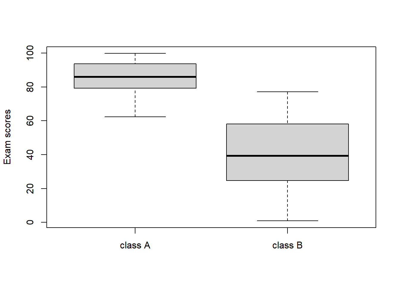
We will start by using a couple of these words in the context of Capstone-style data, and you will soon learn they are all about context. Let’s say you have summative assessment results from two classes of kids, class A and class B. Let’s take a look at their scores:

classA <- rtruncnorm(30, 0, 100, 90, 10)

classB <- rtruncnorm(30, 0, 100, 40, 20)

boxplot(classA, classB, names = c("class A", "class B"), ylab = "Exam scores")

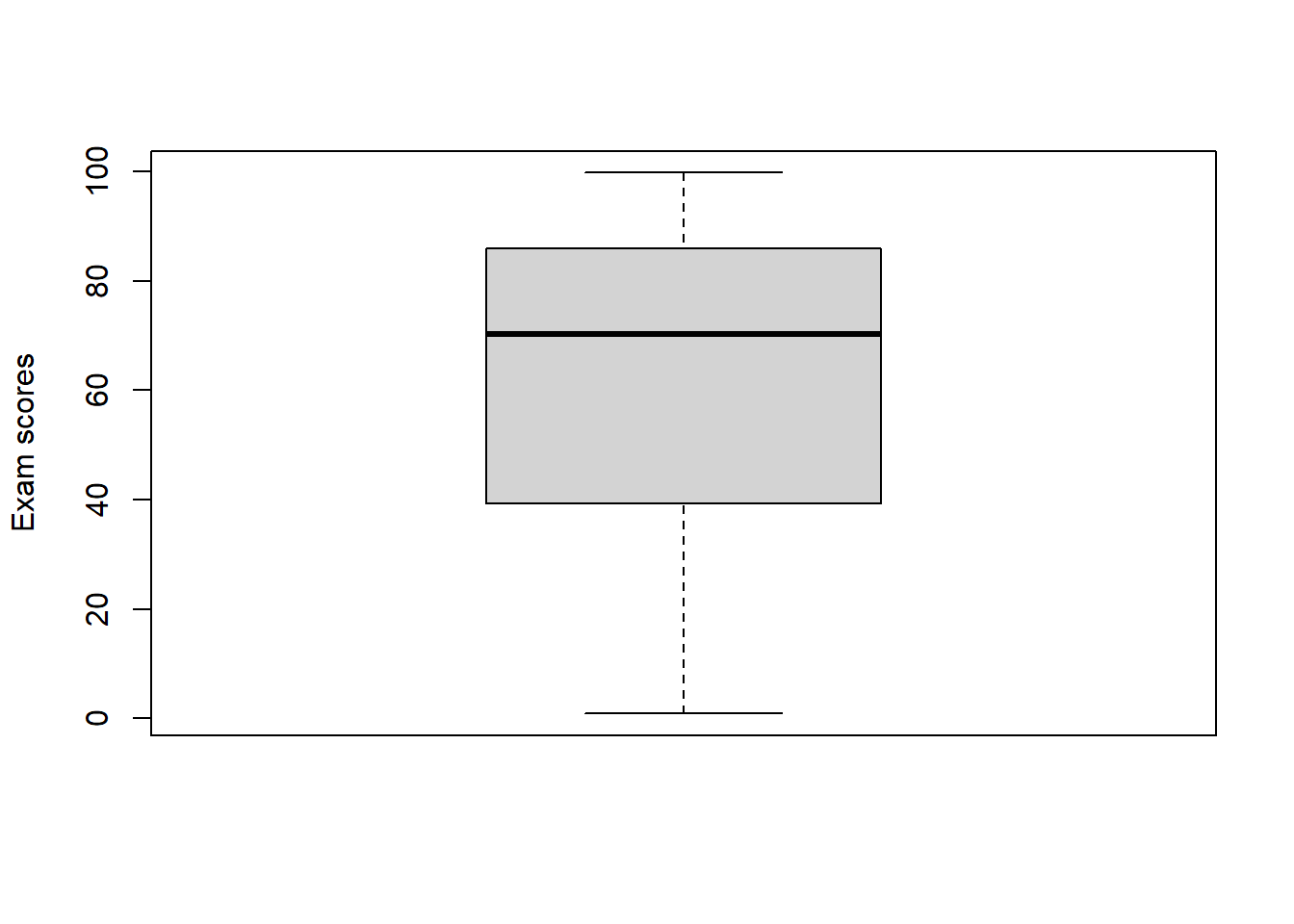
One way on conceptualizing these data is to say that the population (the group that we want to make inference about) is the district-wide collection of all students in this same grade. In this case, class A and class B represents samples from that population. Continuing down this road, what can we learn about our population (or, what inference can we draw) from the two samples? Turns out this is probably not a good idea for most education data, but let’s do it wrong anyway. What if class A was all the data we had? We might say something absurd about how our sample of students suggest that, overall, the grade level is demonstrating high achievement and we can all go home. If all we had was class B, we would conclude the opposite. If we did something really nuts like combining the scores into one larger sample:

boxplot(c(classA, classB), names = c("combined classes"), ylab = "Exam scores")

then we might start talking about ’very disparate achievement levels that suggest the need for remediation for our lowest-achieving students.

The problem here is that we have really, really good reason to believe that these two samples are not random samples from the population, i.e., they are not representative of the population. You can think of dozens and dozens of reasons why students get assigned to schools, and to teachers within schools, and to sections within teachers such that you end up with the opposite of a random sample. If the gods of fortune actually smiled down upon you and you do have random samples, the above logic is actually legitimate and gets used all the time.

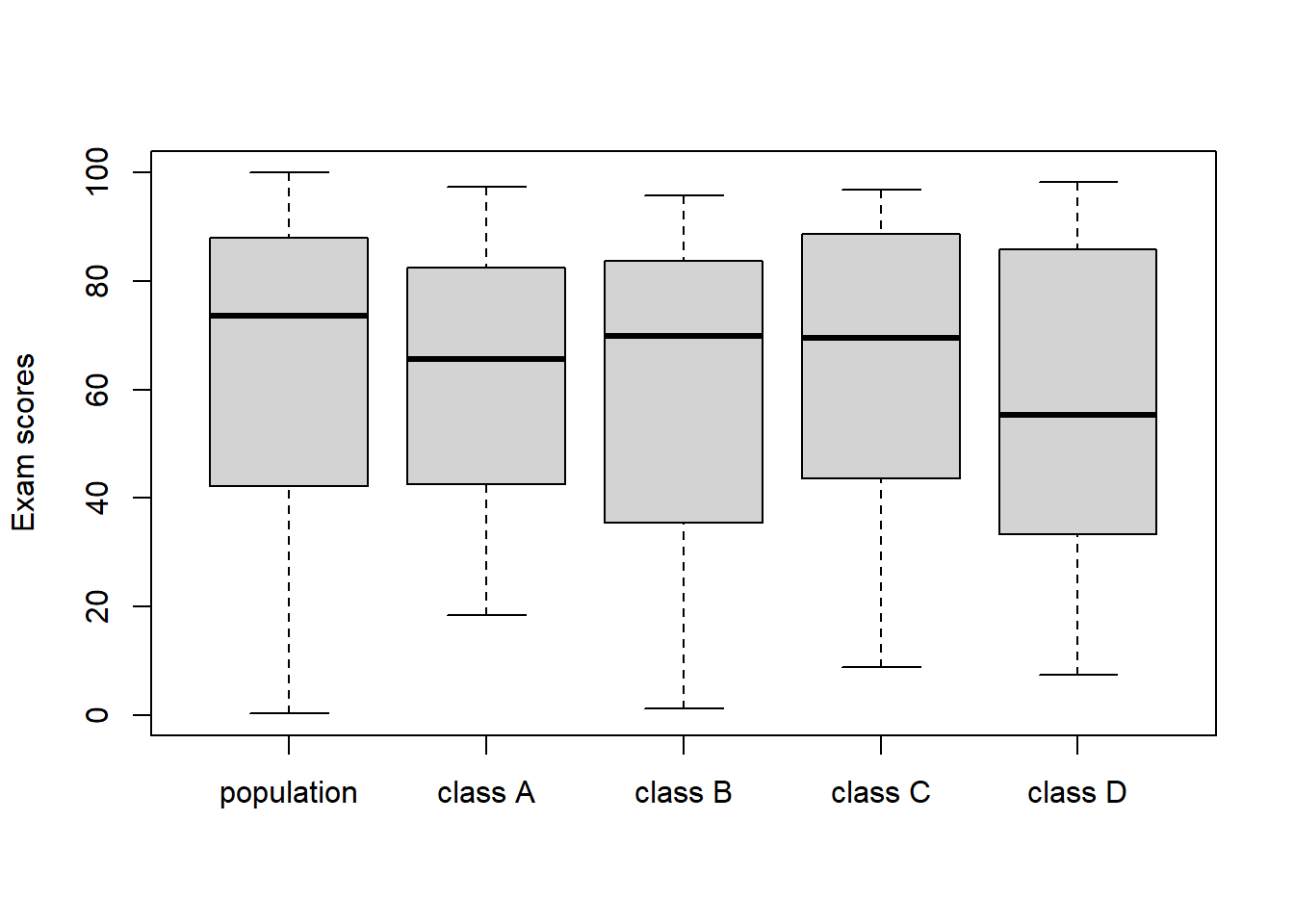
For example, I am going to generate exam scores for 1000 students. Then, I am going to take 4 random samples of 30 students (representing 4 classrooms of students) from that population and see how it shakes out.

population <- c(rtruncnorm(500, 0, 100, 90, 10), rtruncnorm(500, 0, 100, 40, 20))

indices1 <- sample(1:1000, 30); class1 <- population[indices1] 
indices2 <- sample((1:1000)[-indices1], 30); class2 <- population[indices2]
indices3 <- sample((1:1000)[-c(indices1, indices2)], 30); class3 <- population[indices3]
indices4 <- sample((1:1000)[-c(indices1, indices2, indices3)], 30); class4 <- population[indices4]

boxplot(population, class1, class2, class3, class4, names = c("population", "class A", "class B", "class C", "class D"), ylab = "Exam scores")

That worked surprisingly well. If the sample is a good representation of the population, then it seems like we can learn something about the population from the sample. Ergo, the basis of polling, epidemiology, etc.

Like we talked about, this very rarely applies to education data. So, what are your alternatives in this situation?

Recall that you have two classes, class A and B. Options include:

Define your population as all of the students of the same grade in your school, rather than the district, and class A and class B as samples from this population. However, this has the same problems as above: how realistic is it that your classes represent a random sample of all kids in the same grade?
Define your population as all of the students that you teach of the same grade in your school, rather than the entire school, and class A and class B as samples from this population. Now this is getting ridiculous, but how realistic is it that your classes represent a random sample of all kids that you teach?
Define your samples as your population(s). Rather than trying to make inference to a larger population that is inappropriate and likely to get you in trouble, keep your inference where it probably belongs: on the kids you are actually working with.

This seems like an exercise in the obvious, but it has real implications for how you talk about your data. Implications are:

if class A and class B are very different in terms of achievement levels (i.e., a non-random sample), you should probably not be comparing summative assessment scores (and you should encourage your admins to stop doing it too)
if you cannot compare class A and class B, then your best option is to work at the level of the individual student and start talking about how much individuals improve

We are dancing around the concept of unit of observation and what is most appropriate for you folks. If you treat your classes as the unit of observation, then you inevitably end up comparing summative assessments across classes and that can be a real problem. If, on the other hand, you treat the student as the unit of observation you can start making inference about how much students improve from a pre-test to a summative test, or from unit 1 to unit 2, etc.

Technical sidenote: be really thoughtful about how you measure gains in students. If student A has a pre-test score of 40% and a summative test score of 70% (a change of 30%), and student B has a pre-test score of 70% and a summative test score of 100% (a change of 30%), using the 30% as metrics is real problematic because it reduces those two individuals to the same score. Despite the fact that those are two very different kids. A better metric is one that most of you know already, the normalized gain:

\[\textrm{normalized gain} = \frac{\textrm{post-test score} - \textrm{pre-test score}}{100 - \textrm{pre-test score}}\] This changes an exam score into the difference between the scores (numerator) and the amount the student could improve (denominator), and it expresses the achievement of a student relative to the level of knowledge when the pre-test was given. Use this. Back to our example, the first student would have a normalized gain of:

\[\textrm{normalized gain} = \frac{\textrm{70} - \textrm{40}}{100 - 40} = 0.5\] i.e., that student made up half of the gap. The second student would have a normalized gain of:

\[\textrm{normalized gain} = \frac{\textrm{100} - \textrm{70}}{100 - 70} = 1\]

i.e., that student made up the entire gap.

2.3 How to mess up

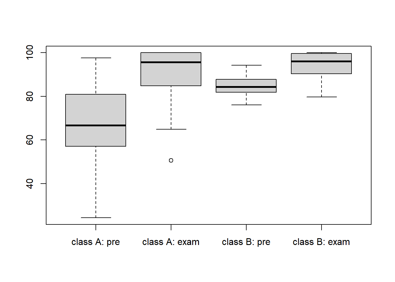
Let’s demonstrate what not to do! I am going to generate pre-test scores and summative exam scores for two classes, class A and class B, over a unit on stratigraphy. Class A got to do the “treatment”: they got go outside, climb over road cuts and break rocks. Class B got to do traditional book and movie work.

classA_pretest <- rtruncnorm(30, 0, 100, 70, 20)
classA_posttest <- sapply(classA_pretest + runif(30, 25, 35), function(x) min(x, 100))

classB_pretest <- rtruncnorm(30, 0, 100, 85, 5)
classB_posttest <- sapply(classB_pretest + runif(30, 0, 20), function(x) min(x, 100))

boxplot(classA_pretest, classA_posttest, classB_pretest, classB_posttest, 
        names = c("class A: pre", "class A: exam", "class B: pre", "class B: exam"))

Here is a really bad job (I have seen this a lot):

The mean summative exam score for class B (96.81) was slightly higher than for class A (90.97), suggesting the treatment did not result in any differences in content mastery.

Another bad job:

The mean summative exam score for class B (96.81) was slightly higher than for class A (90.97), and the range of scores for class B was narrower than for class A. Combined, these results suggest the treatment did not result in any differences in content mastery.

Marginally better:

Although the comparisons of mean summative exam score for class B (96.81) to class A (90.97), and the range of scores for class B to class A suggest that there the treatment did not result in overall higher mastery, inspection of the pre-test scores suggest this comparison is problematic. Going into the unit, class B had a significant head start on class A: the median, first and third quartiles for class B exceeded the third quartile for class A, indicating that 75% of students in class B exceeded all but the top 25% of class A.

Better:

Pre-test scores strongly suggested that class A and class B were comprised of students with very different achievement levels (…insert your comparison using median, means, or quartiles here…), indicating that a cross-class comparison of summative scores was inappropriate. Using normalized gains as a metric, I found that the average normalized gain for class A was 0.82, compared to an average normalized gain of 0.81 for class B. More importantly, these results suggest dramatic within-individual improvement in class A given that the minimum normalized gain was … Finally, I note that the scores within class A demonstrated a much more significant shift than class B, as nearly all of the lowest-achieving students demonstrated content mastery on the summative assessment. Combined, these results suggest …

This does not get you out of the box of having to talk about all the other reasons why the improvement could have occurred (e.g., better snacks for class A, remedial help, classroom volunteers), but it is a much clearer treatment of your data.

The lessons to learn here:

think hard about what inference you want to make/is appropriate (thereby defining your sample and population)
think hard about what your unit of observation is
think hard about what a fair comparison is for your kids
think very hard about paying attention to your lowest-performing kids and their improvements
it is very easy for means and medians to mask individual improvement that could be really powerful, i.e., concluding that treatments only appeared to work for English-language learners is a really powerful conclusion.

2.4 Case study 2

Here is a short assignment you can use to show me how well you understand these ideas. Here is the set-up:

A teacher has two sections of students (section 1 and section 2), and wants to investigate the impact of a particular teaching modality on content mastery and has the space in the schedule to work with two unrelated units (unit A and unit B). The teacher has decided to treat unit A as a comparison group (standard teaching) and unit B as a treatment group (fancy teaching). For both units, the teacher conducted a pre-test followed by a summative assessment. The data are here.

Using one figure and a short, concise (1/2 page single spaced, no more) summary, please describe what these data tell you about the teaching method.

Please do be careful, you have to at least mention that these units cover different topics.