Part 4 Caution, for there be dragons
There is no analysis for this final part of the course. Rather, it is a note of caution and hope, followed by a short summary of a really compelling argument. There is an understandable desire to use heavy-duty stuff to analyze your Capstone data; it looks cool, makes you seem awesome, and tends to make your audience believe that you really know what you are talking about. “Tests” that may sound familiar are the “t-test” (of which there are multiple versions), “chi-square” tests, “ANOVA,” and a series of other scary-sounding terms.
When used appropriately and in the correct context, these tools can be a powerful way to uncover patterns and relationships in your data, and to assess the probability that your results are due to chance alone. However, in the context of Capstone-style research they are NOT a required component of your analysis. I am here to disabuse you of that notion, and to convince you that good graphs and writing can tell almost the same story.
Let’s simulate some pre-unit and summative assessment data for a single class with 35 students.
pre_scores <- rtruncnorm(35, 0, 100, 70, 15)
post_scores <- sapply(pre_scores + runif(35, 5, 35), function(x) min(x, 100))

boxplot(pre_scores, post_scores, names = c("pre-unit assessment", "summative assessment"), ylab = "Exam scores")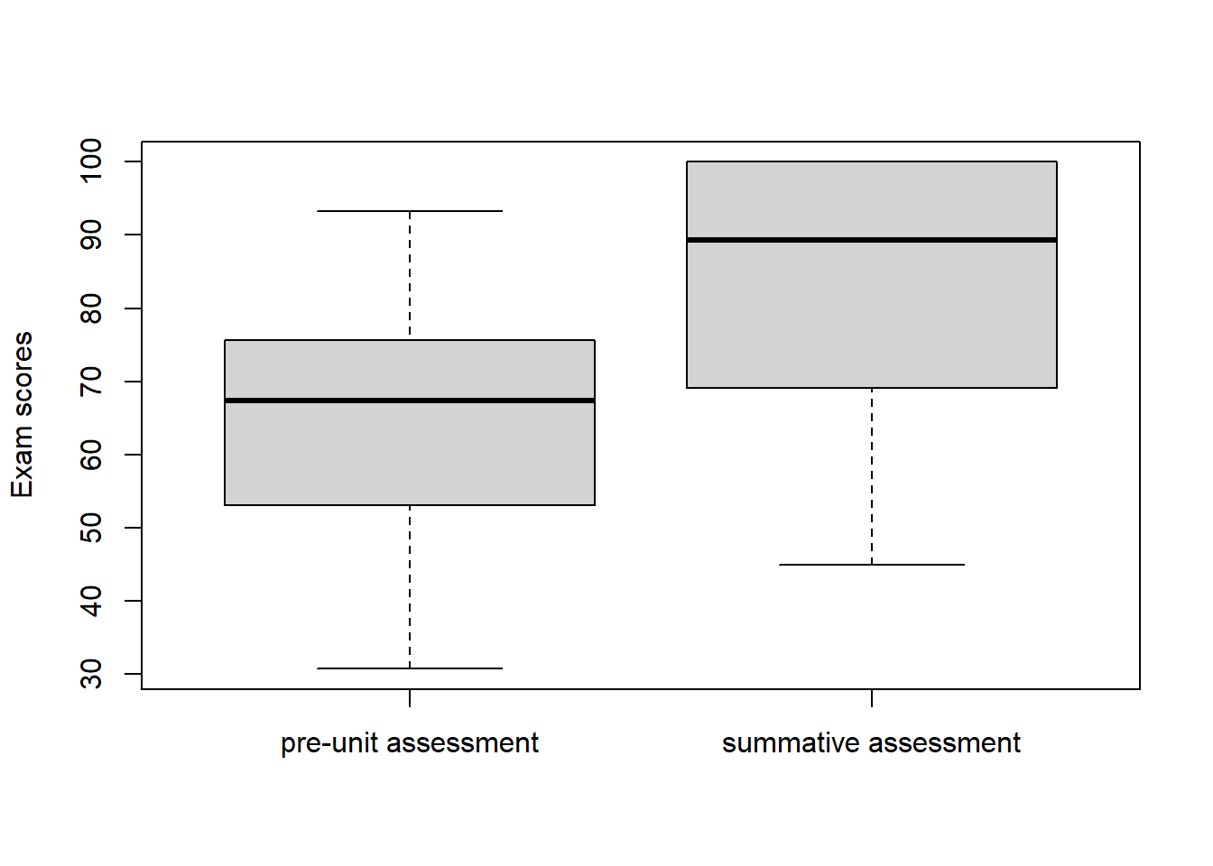
What would a good description of these data look like?
I found a large difference in the median value of the summative assessment (83.8514), compared to the pre-unit assessment (65.5). Moreover, a comparison of the first quartiles (summative assessment = 71.77; pre-unit assessment = 53.87) strongly indicated that the change in medians also reflected an improvement amongst the lowest-achieving students. Of those students that scored less than a 70% on the pre-unit assessment, 63 percent of them had improved to above a 70% by the summative assessment.
That tells a good story. You are honest by showing a graph of the two sets of scores so that your reader gets a clear picture. You don’t just use a mean (or median) value, and you back up your conclusion about your median shift by saying that improvements were felt across all achievement levels.
What does a t-test add to that description? Discounting some honest work that needs to go into evaluating whether you can use a particular test or not (and they all have assumptions that need to be checked), here is what that would look like absent all context:
t_test <- t.test(post_scores, pre_scores, paired = TRUE)
t_test
##
## Paired t-test
##
## data: post_scores and pre_scores
## t = 11.585, df = 34, p-value = 2.371e-13
## alternative hypothesis: true difference in means is not equal to 0
## 95 percent confidence interval:
## 14.49899 20.66816
## sample estimates:
## mean of the differences
## 17.58358What does that output tell you? Pay attention to the p-value = part of that output. That essentially tells you that the probability of you observing the improvement that you did if there were actually no difference between the scores is less than really small, or bascially zero. This is a hypothesis significance test; you make a claim about the world (null hypothesis) and then evaluate the probability of seeing your result if that null hypothesis were true. So, in this case if there were no difference between the scores the probability of you seeing your result is basically zero. You conclude by “rejecting the null,” i.e., your result is so weird if the null were true that the null cannot be true. Strange logic, right?
How does that add value to your conclusion? Here would be one method:
I found a large difference in the median value of the summative assessment (83.8514), compared to the pre-unit assessment (65.5). A paired t-test indicated that the probability of this result being due to chance was essentially zero (paired t-test: t = 13, df = 34, p < 0.001). Moreover, a comparison of the first quartiles (summative assessment = 71.77; pre-unit assessment = 53.87) strongly indicated that the change in medians also reflected an improvement amongst the lowest-achieving students. Of those students that scored less than a 70% on the pre-unit assessment, 63 percent of them had improved to above a 70% by the summative assessment.
I suggest that for most of you and your data, this does not add all that much to an otherwise solid, thorough, and honest description of these results.
I want to be clear that I am not discounting the use of “heavy-duty” stuff; I collect my paycheck by doing (to my way of thinking) mind-bogglingly complicated analyses. And it is fun for me. It allows me to understand nature better than I would have been able to otherwise. However, it seldom provides any more clarity than good, descriptive summaries of that data. It “merely” adds rigor and nuance.
4.1 A final exercise and a warning
This idea of “null hypothesis significance testing” (remember, a null hypothesis is the way you think the world works, and the significance testing part tells you how likely you are to see your data if the null hypothesis were true) has been heavily challenged for educational research. Here is a quote from a seminal article on the subject (Kirk 1996):
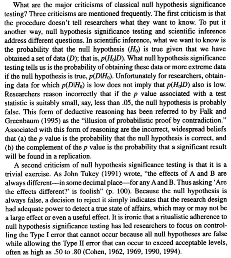
Here is my final challenge to you. I want you to really struggle with this quote. All of you have training in sciences, but this language is going to be unfamiliar to some. Read this quote, ask questions of me and your colleagues in our online Discussion forums, and, when you are ready, write a half-page to the following prompt:
From whatever baseline of science training you have, please re-state in your own words and then summarize these first two objections to the “heavy-duty” stuff, or null hypothesis significance testing.
There are a multiverse of possible good ways to respond to this from whatever level of training you have in the sciences. I more want to hear your critical thinking than I do a preconceived notion of what you should know. The bottom line is: it is okay for you to not use the heavy stuff.
References
Kirk, R. E. (1996). Practical Significance: A Concept Whose Time Has Come. Educational and Psychological Measurement, 56(5), 746–759. https://doi.org/10.1177/0013164496056005002