Chapter 11 The tidyr package
11.1 What is tidyr?
The same data can be organized (or structured) in multiple ways. However, one special structure of data, called tidy data, is particularly useful for data modeling and visualization. In fact, every function in
tidyverseexpects your data to be organized as tidy data. The term tidy data provide a framework for organizing your data that conform to standards that make data easier to use. Tidy data may still require further efforts for actual data modeling and visualization, but the job will be much easier. Hadley Wickham wrote a paper about tidy data, and you can find it here.The official tidyverse website (https://tidyr.tidyverse.org/) introduces the
tidyrpackage as follows:
"The goal of tidyr is to help you create tidy data. Tidy data is data where:
- Every column is variable.
- Every row is an observation.
- Every cell is a single value.
Tidy data describes a standard way of storing data that is used wherever possible throughout the tidyverse. If you ensure that your data is tidy, you’ll spend less time fighting with the tools and more time working on your analysis. Learn more about tidy data in vignette(“tidy-data”)."
- The definition of tidy data requires the definitions of variables and observations. Hadley’s paper present the definition as follows:
“A dataset is a collection of values, usually either numbers (if quantitative) or strings (if qualitative). Values are organised in two ways. Every value belongs to a variable and an observation. A variable contains all values that measure the same underlying attribute (like height, temperature, duration) across units. An observation contains all values measured on the same unit (like a person, or a day, or a race) across attributes.”
- It is important to keep in mind that the definition of a variable might be changed depending on your purpose (from A Tidyverse Cookbook):
“As you work with data, you will be surprised to realize that what is a variable (or observation) will depend less on the data itself and more on what you are trying to do with it. With enough mental flexibility, you can consider anything to be a variable. However, some variables will be more useful than others for any specific task.”
- This lecture focuses four key functions in the
tidyrpackage:pivot_longer()lengthens data, increasing the number of rows and decreasing the number of columns (i.e., turning columns into rows)pivot_wider()widens data, increasing the number of columns and decreasing the number of rows (i.e., turning rows into columns)separate()separates a character column into multiple columns with a regular expression or numeric locationsunite()unites multiple columns into one by pasting strings together
11.2 An example
iris“gives the measurements in centimeters of the variables sepal length and width and petal length and width, respectively, for 50 flowers from each of 3 species of iris. The species are Iris setosa, versicolor, and virginica.”
# as_tibble() convert a data frame into a tibble
# recall the definition of tidy data
#   - Every column is variable
#   - Every row is an observation
#   - Every cell is a single value
# Does the iris data satisfy the three conditions?
as_tibble(iris)
## # A tibble: 150 x 5
## Sepal.Length Sepal.Width Petal.Length Petal.Width Species
## <dbl> <dbl> <dbl> <dbl> <fct>
## 1 5.1 3.5 1.4 0.2 setosa
## 2 4.9 3 1.4 0.2 setosa
## 3 4.7 3.2 1.3 0.2 setosa
## 4 4.6 3.1 1.5 0.2 setosa
## 5 5 3.6 1.4 0.2 setosa
## 6 5.4 3.9 1.7 0.4 setosa
## 7 4.6 3.4 1.4 0.3 setosa
## 8 5 3.4 1.5 0.2 setosa
## 9 4.4 2.9 1.4 0.2 setosa
## 10 4.9 3.1 1.5 0.1 setosa
## # ... with 140 more rows- Suppose that you need to create the following figure using
ggplot2.- Recall your
ggplot2class and sketch the code - Is there any issue in the
irisdata that prevents you from writing the code?
- Recall your
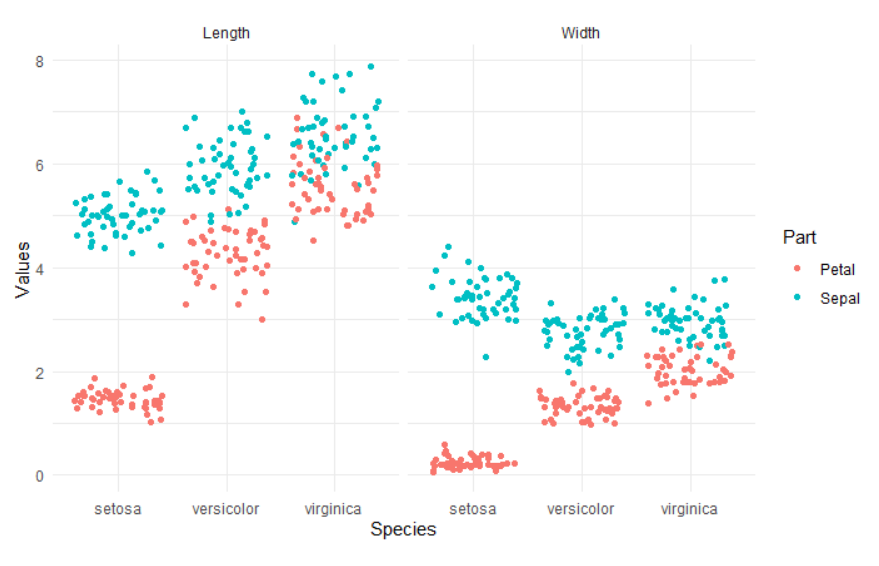
- In order to easily create the figure above, you need to reorganize (or restructure or reshape) the
irisdata as the following:
# STEP 1: pivot_longer() lengthens data
iris %>%
  pivot_longer(cols = -Species, names_to = "Measures", values_to = "Values")
## # A tibble: 600 x 3
## Species Measures Values
## <fct> <chr> <dbl>
## 1 setosa Sepal.Length 5.1
## 2 setosa Sepal.Width 3.5
## 3 setosa Petal.Length 1.4
## 4 setosa Petal.Width 0.2
## 5 setosa Sepal.Length 4.9
## 6 setosa Sepal.Width 3
## 7 setosa Petal.Length 1.4
## 8 setosa Petal.Width 0.2
## 9 setosa Sepal.Length 4.7
## 10 setosa Sepal.Width 3.2
## # ... with 590 more rows# STEP 2: `separate()` separates a character column into multiple columns
# recall the definition of tidy data
# - Every column is variable
# - Every row is an observation
# - Every cell is a single value
# Does this reorganized iris data satisfy the three conditions?
iris %>%
pivot_longer(cols = -Species, names_to = "Measures", values_to = "Values") %>%
separate(col = Measures, into = c("Part", "Measure"))## # A tibble: 600 x 4
## Species Part Measure Values
## <fct> <chr> <chr> <dbl>
## 1 setosa Sepal Length 5.1
## 2 setosa Sepal Width 3.5
## 3 setosa Petal Length 1.4
## 4 setosa Petal Width 0.2
## 5 setosa Sepal Length 4.9
## 6 setosa Sepal Width 3
## 7 setosa Petal Length 1.4
## 8 setosa Petal Width 0.2
## 9 setosa Sepal Length 4.7
## 10 setosa Sepal Width 3.2
## # ... with 590 more rows# STEP 3: `ggplot()` creates the plot
# Can you see the advantage of the reorganized iris data?
iris %>%
pivot_longer(cols = -Species, names_to = "Measures", values_to = "Values") %>%
separate(col = Measures, into = c("Part", "Measure")) %>%
ggplot(aes(x = Species, y = Values, color = Part)) +
geom_jitter() +
facet_grid(cols = vars(Measure)) +
theme_minimal()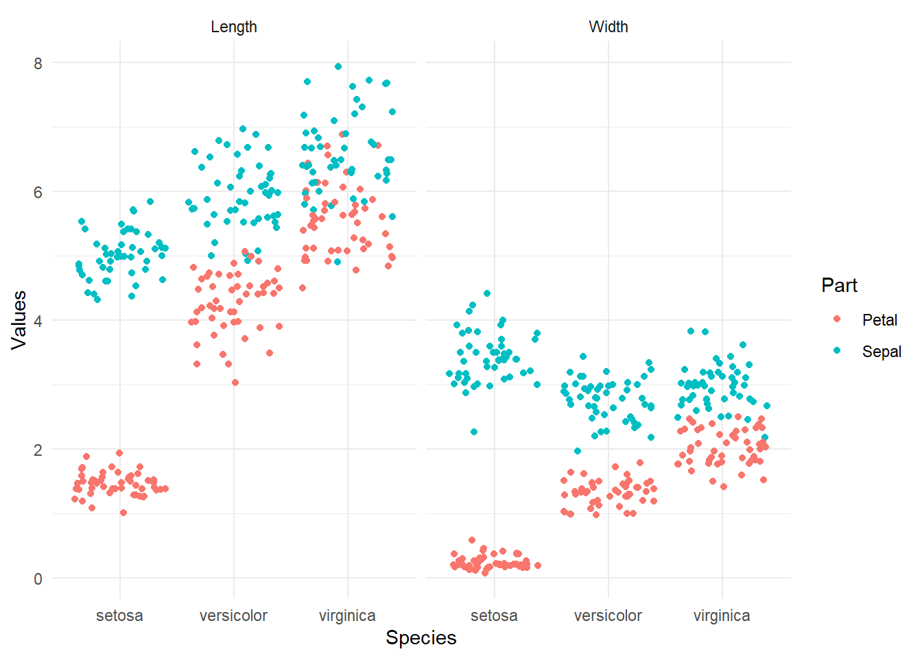
11.3 pivot_longer()
“A common problem is a dataset where some of the column names are not names of variables, but values of a variable. Take table4a: the column names 1999 and 2000 represent values of the year variable, the values in the 1999 and 2000 columns represent values of the cases variable, and each row represents two observations, not one.” (from 12.3 Pivoting in R for Data Science)
## # A tibble: 3 x 3
##   country     `1999` `2000`
## * <chr>        <int>  <int>
## 1 Afghanistan    745   2666
## 2 Brazil       37737  80488
## 3 China       212258 213766
"To tidy a dataset like this, we need to pivot the offending columns into a new pair of variables. To describe that operation we need three parameters:
- The set of columns whose names are values, not variables. In this example, those are the columns 1999 and 2000.
- The name of the variable to move the column names to. Here it is year.
- The name of the variable to move the column values to. Here it’s cases.
Together those parameters generate the call to pivot_longer():"
## # A tibble: 6 x 3
##   country     year   cases
##   <chr>       <chr>  <int>
## 1 Afghanistan 1999     745
## 2 Afghanistan 2000    2666
## 3 Brazil      1999   37737
## 4 Brazil      2000   80488
## 5 China       1999  212258
## 6 China 2000 213766- Usage
- pivot_longer(data, cols, names_to, values_to)
- cols =
columns to pivot into longer format - names_to = A string specifying the name of the column to create from the data stored in the column names of data
- values_to = A string specifying the name of the column to create from the data stored in cell values
- cols =
- check here for the full usage.
- pivot_longer(data, cols, names_to, values_to)
- Exercise 1
relig_income is a tibble in tidyr which contains the result of religion and income survey.
## # A tibble: 18 x 11
##    religion `<$10k` `$10-20k` `$20-30k` `$30-40k` `$40-50k` `$50-75k` `$75-100k`
##    <chr>      <dbl>     <dbl>     <dbl>     <dbl>     <dbl>     <dbl>      <dbl>
##  1 Agnostic      27        34        60        81        76       137        122
##  2 Atheist       12        27        37        52        35        70         73
##  3 Buddhist      27        21        30        34        33        58         62
##  4 Catholic     418       617       732       670       638      1116        949
##  5 Don’t ~       15        14        15        11        10        35         21
##  6 Evangel~     575       869      1064       982       881      1486        949
##  7 Hindu          1         9         7         9        11        34         47
##  8 Histori~     228       244       236       238       197       223        131
##  9 Jehovah~      20        27        24        24        21        30         15
## 10 Jewish        19        19        25        25        30        95         69
## 11 Mainlin~     289       495       619       655       651      1107        939
## 12 Mormon        29        40        48        51        56       112         85
## 13 Muslim         6         7         9        10         9        23         16
## 14 Orthodox      13        17        23        32        32        47         38
## 15 Other C~       9         7        11        13        13        14         18
## 16 Other F~      20        33        40        46        49        63         46
## 17 Other W~       5         2         3         4         2         7          3
## 18 Unaffil~     217       299       374       365       341       528        407
## # ... with 3 more variables: $100-150k <dbl>, >150k <dbl>,
## #   Don't know/refused <dbl>
Is relig_income a tidy data? why?
If not, tidy relig_income.
- Exercise 2
Let’s create an hypothetical stocks data which contains the prices of three stocks.
stocks <- tibble(
  time = as.Date('2009-01-01') + 0:1,
  Stock_X = c(1000,1200),
  Stock_Y = c(900,1000),
  Stock_Z = c(1400,1000)
)
stocks
## # A tibble: 2 x 4
## time Stock_X Stock_Y Stock_Z
## <date> <dbl> <dbl> <dbl>
## 1 2009-01-01 1000 900 1400
## 2 2009-01-02 1200 1000 1000Is stocks tidy? why?
If not, tidy stocks.
## # A tibble: 6 x 3
##   time       stock   price
##   <date>     <chr>   <dbl>
## 1 2009-01-01 Stock_X  1000
## 2 2009-01-01 Stock_Y   900
## 3 2009-01-01 Stock_Z  1400
## 4 2009-01-02 Stock_X  1200
## 5 2009-01-02 Stock_Y  1000
## 6 2009-01-02 Stock_Z 1000- Exercise 3
billboard is a data set in tidyr. This is an typical example of a longitudinal data in a wide form.
## # A tibble: 317 x 79
##    artist   track   date.entered   wk1   wk2   wk3   wk4   wk5   wk6   wk7   wk8
##    <chr>    <chr>   <date>       <dbl> <dbl> <dbl> <dbl> <dbl> <dbl> <dbl> <dbl>
##  1 2 Pac    Baby D~ 2000-02-26      87    82    72    77    87    94    99    NA
##  2 2Ge+her  The Ha~ 2000-09-02      91    87    92    NA    NA    NA    NA    NA
##  3 3 Doors~ Krypto~ 2000-04-08      81    70    68    67    66    57    54    53
##  4 3 Doors~ Loser   2000-10-21      76    76    72    69    67    65    55    59
##  5 504 Boyz Wobble~ 2000-04-15      57    34    25    17    17    31    36    49
##  6 98^0     Give M~ 2000-08-19      51    39    34    26    26    19     2     2
##  7 A*Teens  Dancin~ 2000-07-08      97    97    96    95   100    NA    NA    NA
##  8 Aaliyah  I Don'~ 2000-01-29      84    62    51    41    38    35    35    38
##  9 Aaliyah  Try Ag~ 2000-03-18      59    53    38    28    21    18    16    14
## 10 Adams, ~ Open M~ 2000-08-26      76    76    74    69    68    67    61    58
## # ... with 307 more rows, and 68 more variables: wk9 <dbl>, wk10 <dbl>,
## #   wk11 <dbl>, wk12 <dbl>, wk13 <dbl>, wk14 <dbl>, wk15 <dbl>, wk16 <dbl>,
## #   wk17 <dbl>, wk18 <dbl>, wk19 <dbl>, wk20 <dbl>, wk21 <dbl>, wk22 <dbl>,
## #   wk23 <dbl>, wk24 <dbl>, wk25 <dbl>, wk26 <dbl>, wk27 <dbl>, wk28 <dbl>,
## #   wk29 <dbl>, wk30 <dbl>, wk31 <dbl>, wk32 <dbl>, wk33 <dbl>, wk34 <dbl>,
## #   wk35 <dbl>, wk36 <dbl>, wk37 <dbl>, wk38 <dbl>, wk39 <dbl>, wk40 <dbl>,
## #   wk41 <dbl>, wk42 <dbl>, wk43 <dbl>, wk44 <dbl>, wk45 <dbl>, wk46 <dbl>,
## #   wk47 <dbl>, wk48 <dbl>, wk49 <dbl>, wk50 <dbl>, wk51 <dbl>, wk52 <dbl>,
## #   wk53 <dbl>, wk54 <dbl>, wk55 <dbl>, wk56 <dbl>, wk57 <dbl>, wk58 <dbl>,
## #   wk59 <dbl>, wk60 <dbl>, wk61 <dbl>, wk62 <dbl>, wk63 <dbl>, wk64 <dbl>,
## #   wk65 <dbl>, wk66 <lgl>, wk67 <lgl>, wk68 <lgl>, wk69 <lgl>, wk70 <lgl>,
## #   wk71 <lgl>, wk72 <lgl>, wk73 <lgl>, wk74 <lgl>, wk75 <lgl>, wk76 <lgl>
The following code makes billboard longer.
billboard %>%
  pivot_longer(
    cols = starts_with("wk"),
    names_to = "week",
    values_to = "rank",
    values_drop_na = TRUE
  )
## # A tibble: 5,307 x 5
## artist track date.entered week rank
## <chr> <chr> <date> <chr> <dbl>
## 1 2 Pac Baby Don't Cry (Keep... 2000-02-26 wk1 87
## 2 2 Pac Baby Don't Cry (Keep... 2000-02-26 wk2 82
## 3 2 Pac Baby Don't Cry (Keep... 2000-02-26 wk3 72
## 4 2 Pac Baby Don't Cry (Keep... 2000-02-26 wk4 77
## 5 2 Pac Baby Don't Cry (Keep... 2000-02-26 wk5 87
## 6 2 Pac Baby Don't Cry (Keep... 2000-02-26 wk6 94
## 7 2 Pac Baby Don't Cry (Keep... 2000-02-26 wk7 99
## 8 2Ge+her The Hardest Part Of ... 2000-09-02 wk1 91
## 9 2Ge+her The Hardest Part Of ... 2000-09-02 wk2 87
## 10 2Ge+her The Hardest Part Of ... 2000-09-02 wk3 92
## # ... with 5,297 more rows11.4 pivot_wider()
“pivot_wider() is the opposite of pivot_longer(). You use it when an observation is scattered across multiple rows. For example, take table2: an observation is a country in a year, but each observation is spread across two rows.”
## # A tibble: 12 x 4
##    country      year type            count
##    <chr>       <int> <chr>           <int>
##  1 Afghanistan  1999 cases             745
##  2 Afghanistan  1999 population   19987071
##  3 Afghanistan  2000 cases            2666
##  4 Afghanistan  2000 population   20595360
##  5 Brazil       1999 cases           37737
##  6 Brazil       1999 population  172006362
##  7 Brazil       2000 cases           80488
##  8 Brazil       2000 population  174504898
##  9 China        1999 cases          212258
## 10 China        1999 population 1272915272
## 11 China        2000 cases          213766
## 12 China        2000 population 1280428583
To tidy this up, we first analyse the representation in similar way to pivot_longer(). This time, however, we only need two parameters: * The column to take variable names from. Here, it’s type. * The column to take values from. Here it’s count. Once we’ve figured that out, we can use pivot_wider(), as shown programmatically below, and visually in Figure 12.3.
## # A tibble: 6 x 4
##   country      year  cases population
##   <chr>       <int>  <int>      <int>
## 1 Afghanistan  1999    745   19987071
## 2 Afghanistan  2000   2666   20595360
## 3 Brazil       1999  37737  172006362
## 4 Brazil       2000  80488  174504898
## 5 China        1999 212258 1272915272
## 6 China 2000 213766 1280428583- Usage
- pivot_wider(data, names_from, values_from)
- names_from = A string specifying the name of the column to get the name of the output column
- values_from = A string specifying the name of the column to get the cell values from
- check here for the full usage.
- pivot_wider(data, names_from, values_from)
11.5 separate()
separate() separates a single column into multiple columns. By default, separate() will split values whereever it sees a non-alphanumeric characters.
## # A tibble: 6 x 3
##   country      year rate
## * <chr>       <int> <chr>
## 1 Afghanistan  1999 745/19987071
## 2 Afghanistan  2000 2666/20595360
## 3 Brazil       1999 37737/172006362
## 4 Brazil       2000 80488/174504898
## 5 China        1999 212258/1272915272
## 6 China        2000 213766/1280428583
# By default, any non-alphanumeric character will be a delimiter.
table3 %>%
separate(rate, into = c("cases", "population"))## # A tibble: 6 x 4
## country year cases population
## <chr> <int> <chr> <chr>
## 1 Afghanistan 1999 745 19987071
## 2 Afghanistan 2000 2666 20595360
## 3 Brazil 1999 37737 172006362
## 4 Brazil 2000 80488 174504898
## 5 China 1999 212258 1272915272
## 6 China 2000 213766 1280428583# you can specify your own delimiter using sep
# note that the types of cases and population are characters
# separate() keeps the original type
table3 %>%
separate(rate, into = c("cases", "population"), sep = "/")## # A tibble: 6 x 4
## country year cases population
## <chr> <int> <chr> <chr>
## 1 Afghanistan 1999 745 19987071
## 2 Afghanistan 2000 2666 20595360
## 3 Brazil 1999 37737 172006362
## 4 Brazil 2000 80488 174504898
## 5 China 1999 212258 1272915272
## 6 China 2000 213766 1280428583# convert = TRUE will convert to better type
table3 %>%
separate(rate, into = c("cases", "population"), convert = TRUE)## # A tibble: 6 x 4
## country year cases population
## <chr> <int> <int> <int>
## 1 Afghanistan 1999 745 19987071
## 2 Afghanistan 2000 2666 20595360
## 3 Brazil 1999 37737 172006362
## 4 Brazil 2000 80488 174504898
## 5 China 1999 212258 1272915272
## 6 China 2000 213766 1280428583# separate() will interpret the integers as positions to split at
table3 %>%
separate(year, into = c("century", "year"), sep = 2)## # A tibble: 6 x 4
## country century year rate
## <chr> <chr> <chr> <chr>
## 1 Afghanistan 19 99 745/19987071
## 2 Afghanistan 20 00 2666/20595360
## 3 Brazil 19 99 37737/172006362
## 4 Brazil 20 00 80488/174504898
## 5 China 19 99 212258/1272915272
## 6 China 20 00 213766/128042858311.6 unite()
unite() combines multiple columns into a single column.
## # A tibble: 6 x 4
##   country     century year  rate
## * <chr>       <chr>   <chr> <chr>
## 1 Afghanistan 19      99    745/19987071
## 2 Afghanistan 20      00    2666/20595360
## 3 Brazil      19      99    37737/172006362
## 4 Brazil      20      00    80488/174504898
## 5 China       19      99    212258/1272915272
## 6 China 20 00 213766/1280428583## # A tibble: 6 x 3
## country new rate
## <chr> <chr> <chr>
## 1 Afghanistan 19_99 745/19987071
## 2 Afghanistan 20_00 2666/20595360
## 3 Brazil 19_99 37737/172006362
## 4 Brazil 20_00 80488/174504898
## 5 China 19_99 212258/1272915272
## 6 China 20_00 213766/1280428583## # A tibble: 6 x 3
## country new rate
## <chr> <chr> <chr>
## 1 Afghanistan 1999 745/19987071
## 2 Afghanistan 2000 2666/20595360
## 3 Brazil 1999 37737/172006362
## 4 Brazil 2000 80488/174504898
## 5 China 1999 212258/1272915272
## 6 China 2000 213766/1280428583