Chapter 2 Introduction to R
2.1 Data Analysis Report
- Key components of the data analysis report
- Problem(문제)
- A problem is the clear description about the issue that your analysis will address.
- This is what we need to know.
- Background(배경)
- Background is the context in which your problem is framed
- This is what we already know.
- Where and when does the problem arise?
- Who does the problem affect?
- What attempts have been made to solve the problem?
- Relevance(중요성)
- Relevance is the importance of your analysis.
- This is the reason why we need to solve the problem
- What will happen if the problem is not solved?
- Who will be influenced by the consequences of the problem?
- Objective(목적)
- Objective is the purpose of your analysis.
- This is what you will do to find the reasons behind the problem and to propose more effective approaches to tackle the problem.
- The aims of this analysis is to determine (to explore, to investigate, to understand) …
- Data(자료)
- Data are measurements or observations that are collected as a source of information (e.g., numbers, text, audio, video).
- This is what you analyzed
- participants’ demographics (e.g., age, sex, ethnicity), sampling procedures, sample size, data collection procedure
- Methods(방법)
- Methods provide information about the statistical and data-analytic methods
- This is what you did to analyze your data
- missing data, types of data analysis, statistical models, software
- Results(결과)
- This is what you found from your analysis.
- tables
- graphs
- This is what you found from your analysis.
- Discussion/Conclusion(결론)
- Restate your problems and findings for summary
- State your suggestions on the problem based on your findings.
- You should provide evidence to support each of your suggestions. Make clear connection between your suggestions and the supporting evidence in your results.
- (if any) State the limitations of your analysis
- (if any) State directions for future analysis
- State your closing statement highlighting the importance of your analysis
- Problem(문제)
- A problem statement is a paragraph(s) that
- presents the specific problem you will address (problem),
- contextualizes your problem (background),
- highlights the significance of your problem (relevance),
- presents the specific purpose of your work (objective).
- Possible outline 1 (traditional journal article)
- Introduction
- Problems
- Background
- Relevance
- Objectives
- (Background)
- Methods
- Data
- Results
- Discussion
- (Appendix)
- Introduction
- Possible outline 2 (executive summary + traditional journal article body)
- Introduction (executive summary)
- Problems
- Background
- Relevance
- Objective
- Short summary of your results
- Short summary of your suggestions in your discussion
- Body (traditional journal article)
- Data
- Methods
- Results
- Discussion
- (Appendix)
- Introduction (executive summary)
- Possible outline 3 (executive summary + question-oriented body)
- Introduction (executive summary)
- Problems
- Background
- Relevance
- Objective
- Short summary of your results
- Short summary of your suggestions in your discussion
- Body (question-oriented body)
- Data
- Question1
- Methods
- Results
- Discussion
- Question2
- Methods
- Results
- Discussion
- Question3
- Methods
- Results
- Discussion
- Discussion
- (Appendix)
- Introduction (executive summary)
- Your own outline
- You can arrange the key components above (and more components you want) in a way that can effectively deliver your findings. Design your own outline.
- Tips
- Some readers want to just skim your report. Highlight the headlines for those skimmers.
- Too many text descriptions may hide the outline and main results. Maximize readability of your report.
- Appendix is a wonderful tool for placing technical details, output, extra figures and tables, programming codes.
- Evaluation criteria for data science project
- It’s always good to know the criteria your work will be evaluated.
- e.g., A sample rubric (This is just a sample and not a grading rubric for our class)
2.2 Why R?
- R is a language specifically designed for statistical analysis.
- If you visit the R project website(https://www.r-project.org/), then you will find that the first line of the website says “R is a free software environment for statistical computing and graphics.” R is a language specifically designed for statistical analysis. Many researchers first implement their experimental methods in statistics and machine learning using R. So you can use many cutting-edge algorithms in R by downloading many packages in R.
- R provides wonderful tools for publication-quality data visualization.
- Data visualization help you to understand your data and present your findings to others. In this lecture, you will learn
ggplot2package for data visualization.
- Data visualization help you to understand your data and present your findings to others. In this lecture, you will learn
- R provides wonderful tools for data wrangling.
- The ultimate goal of using R is to understand your data using data visualization and modeling. Often, however, you need to spend lots of time to make your raw data into the appropriate form for data visualization and modeling. This process is often called data wrangling, which includes data transformation and data tidying. In R, the
dplyrpackage was developed for data transformation, and thetidyrpackage was developed for data tidying. We will cover bothdplyrand ‘tidyr’ packages in this lecture.
- Data wrangling is an important skill in these days to effectively handle data from diverse sources (e.g., facebook, twitter, fMRI, eyetracker, EEG). For example, many servers store user data in the JSON format for data exchange, and so you need to handle JSON files if you want to use user data for your analysis.
- The ultimate goal of using R is to understand your data using data visualization and modeling. Often, however, you need to spend lots of time to make your raw data into the appropriate form for data visualization and modeling. This process is often called data wrangling, which includes data transformation and data tidying. In R, the
- R has active and supportive communities.
- You can find many useful resources from R communities. For example, the
bookdownis an R package for writing books, and bookdown.org provides useful R books written with thebookdownpackage for free. In the bookdown.org, you will find our textbook for this class, which is R for Data Science.
- You can find many useful resources from R communities. For example, the
- R is a free open source software.
2.3 R vs Python
Python is another great programming language. You can find many interesting debates over R vs Python on the internet. Here is an example.
In short, Python is a general-purpose programming language used for a wide variety of applications (e.g., data science, web development, database), whereas R is a programming language focusing on data science.
One of the goals of this course is to give you an opportunity for exploring R so that you can make a decision about which language is best for your purpose. You may need both languages.
“Generally, there are a lot of people who talk about R versus Python like it’s a war that either R or Python is going to win. I think that is not helpful because it is not actually a battle. These things exist independently and are both awesome in different ways.”
— Hadley Wickham
2.4 RStudio
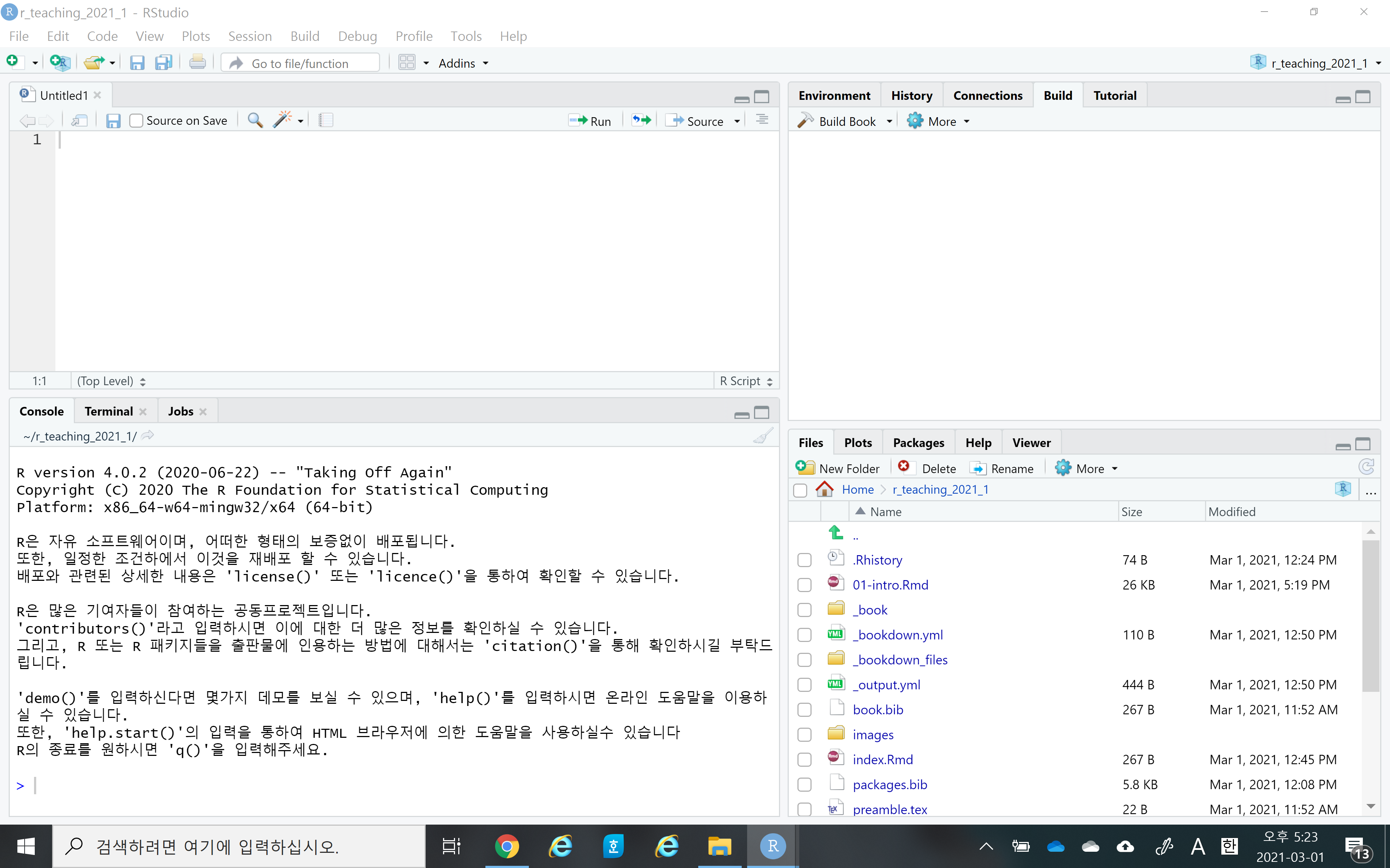
- Once you successfully install R and RStudio, please launch your RStudio. You should see something like the following. Again, the RStudio is a convenient interface (or IDE) for R, and so you only need to launch the RStudio, not R.
Let’s watch a short introductory video for RStudio here
Notice that RStudio consists of four panels (or panes)
- Source editor pane
- This is where you can edit your code in R script or R markdown files
- Console pane
- This is where you can execute your code instantly
- Environment pane
- This is where you can see the objects (or variables)
- File/Plots/Packages/Helps pane
- This is where you can see files, plots, packages, and help documents.
- Source editor pane
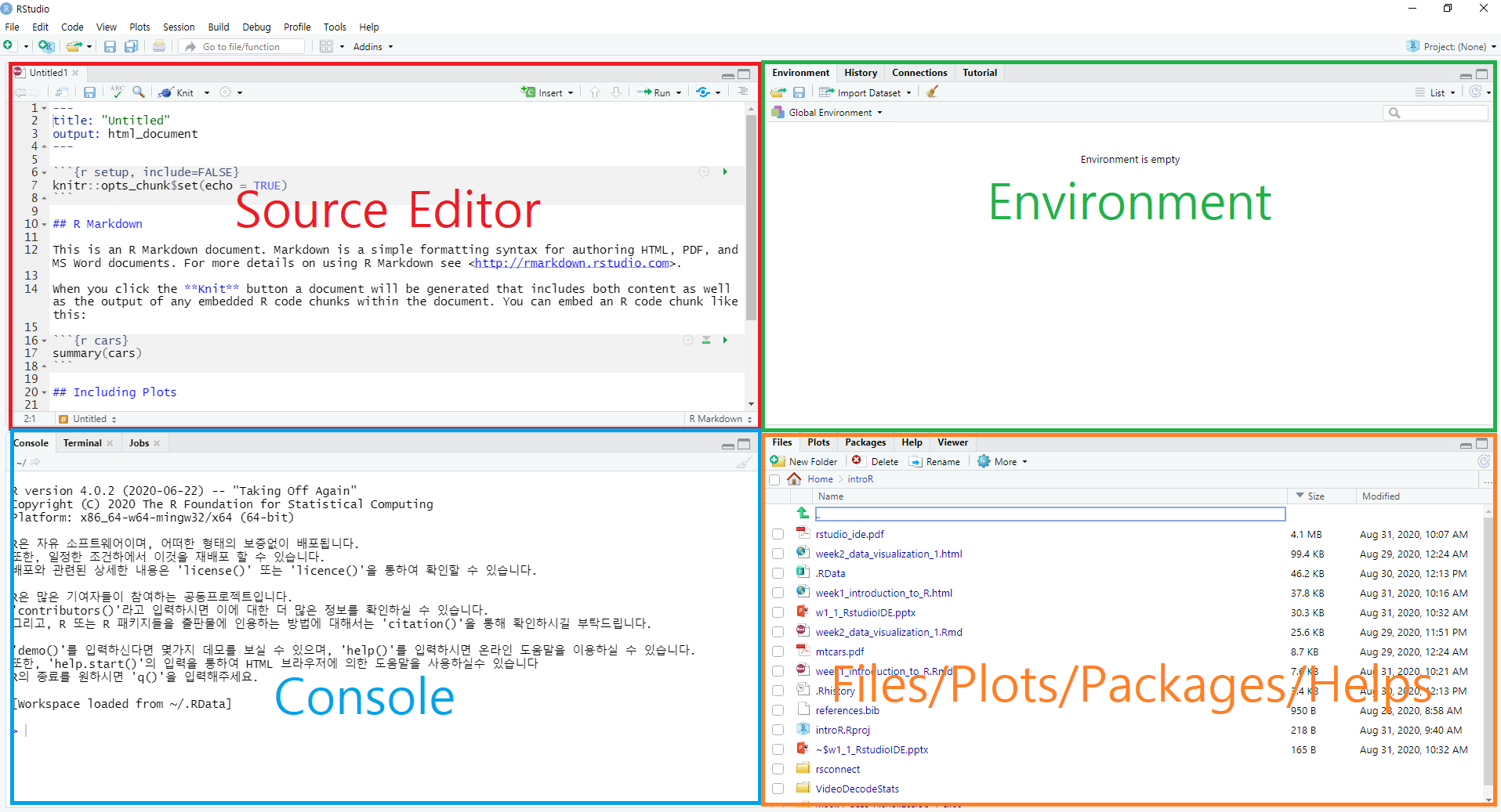
Four main panes in RStudio IDE
- You can find more RStudio features here.
2.5 R Packages
An R package is the collections of functions and data sets developed for a specific purpose. For example, the
carat(short for Classification And REgression Training) package is a package that contains many useful functions for machine learning. We will use thiscaratpackage for our machine learning part in this class.The package system in R is the core part of the R project, and allows any contributor (including you) around the world can contribute to the R project by developing packages.
Currently, the Comprehensive R Archive Network(CRAN) repository contains more than 18,000 packages. A list of R packages are available here.
Installing vs Loading
- Installing means you download the package files from the CRAN repository to your local computer. You may not want to download all the files for the 18,000 packages from the beginning. You may want to download some packages you need into your local computer. You only need to install a package once. An R function named
install.packages()is used to install packages. - Loading means you load functions and data in the package onto your computer memory. Loading functions and data of all packages to memory is inefficient in terms of computers’ memory management. So you only load a package onto memory when you need it. In other word, whenever you want to use functions in a package, you need to load the package that contains the functions. An R function named
library()is used to load packages. - For example, we load the
ggplot2package withlibrary("ggplot2")before using theggplot2functions inggplot(mtcars, aes(x = disp, y = mpg)) + geom_point() + geom_smooth(method = "lm")
- Installing means you download the package files from the CRAN repository to your local computer. You may not want to download all the files for the 18,000 packages from the beginning. You may want to download some packages you need into your local computer. You only need to install a package once. An R function named
2.6 Base R vs Tidyverse
- Base R
- Base R refers to the collection of functions and packages that come with a clean install of R.
- Many packages extend Base R.
- Tidyverse
- The
tidyversepackage(https://www.tidyverse.org) is a collection of packages for more efficient data science in R. - In the
tidyversepackage, thedplyr,tidyr,ggplot2, andpurrrpackages provide many useful functions for efficient data transformation, data tidying, data visualization, and iteration, respectively. - Our textbook R for Data Science (Hadley Wickham) is all about the
tidyversepackage. - The goal of this course is to learn the
tidyversepackage. (The goal of the PART II is to learning the basics of machine learning)
- The
2.7 Console vs R script file vs R Markdown File
For R programming, you need to let computers know what you want them to do for you. Simply, you need to type your R commands. Console, R script file, and R markdown file are three different ways in which you can interact with R.
In the console, you just type the R command at the prompt (i.e.,
>) and press the<Enter>key, then R will execute your commands and show the result. The console allows us to quickly run our commands but the commands will be gone when you quit your R.
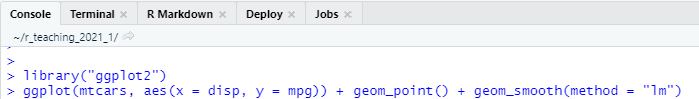
The R Console
- The R script is just a text file having the
.Rfile extension. Using the R script, you can store your R commands for later use. Notice that the R script cannot store your results.
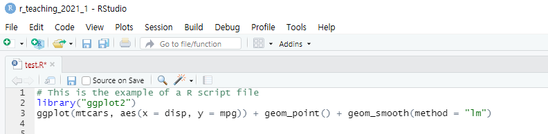
The R script
- The R markdown is also a text file having the
.Rmdfile extension. Using the R markdown, you can store your R commands (gray area), your results, and your texts (white area).
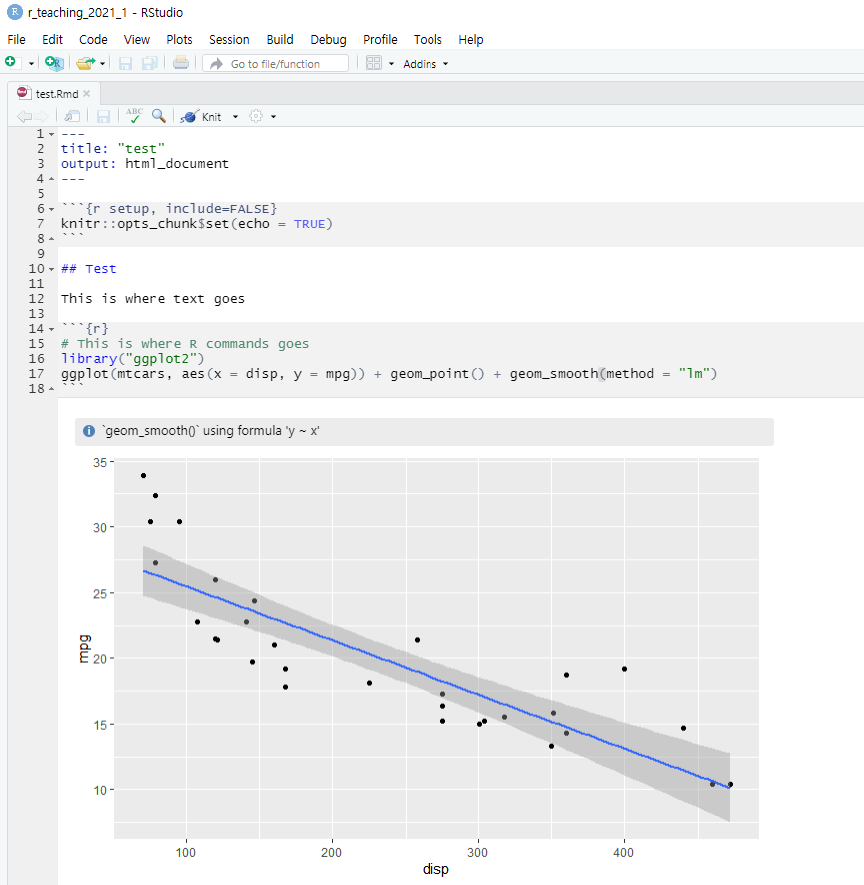
The R markdown
2.8 More about the R makrdown
In this course, we will mainly use the R markdown so that you can learn the advantage of the R markdown. Simply, people use the R markdown because it’s a great tool for communication. In data science, once you analyze your data then you usually want to communicate your findings with others. The R markdown allows you to create documents that include your R codes, results, and texts in a variety of formats such as HTML, PDF, Microsoft Word, and other dynamic documents. It’s a nice example of one-source multi-use.
These days, how you present your work is just as important as what you present. If you learn R markdown, you can present your contents in many different wonderful formats.
This lecture notes was created using the R markdown and then was converted into the html for web lecture notes. More precisely, I used the
bookdownpackage to create this lecture notes. I will introduce thebookdownpackage later in this course so that you can also publish your own lecture notes like this one on the web.Let’s watch a short introductory video for R markdown.
You will be amazed how many nice documents can be created from a simple R markdown text file. Please check nice documents from R markdown here.
If you are serious in R markdown, please read R Markdown: The Definitive Guide(Yihui Xie, J. J. Allaire, Garrett Grolemund).
In this class, we will cover the basic of R markdown.
Let’s explore R markdown a little bit more. You can open a new R markdown template by going
File > New File > R Markdown...
R Markdown template in RStudio
- Notice that R markdown contains white and gray areas. The white area is where your text goes, whereas the gray area is where your R code goes.
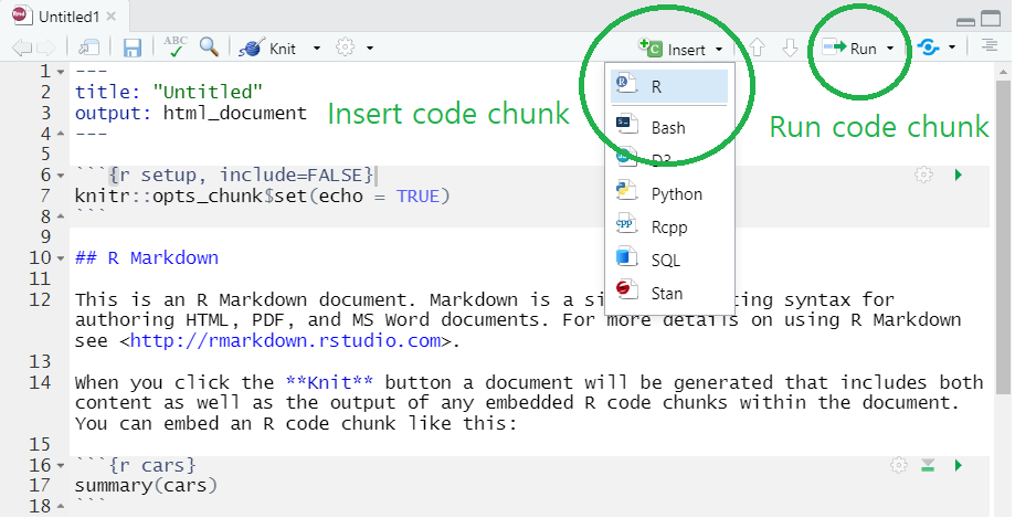
- You can create a code chunk by
- clicking
insertand chooseRon the menu (check the green circle on the above image) or - typing a short cut key or
- Windows:
Ctrl + Alt + I - Mac:
Cmd + Option + I
- Windows:
- clicking
- You can run the code in a code chunk by
- clicking
Runon the menu (check the green circle on the above image) or - typing
Ctrl + Enterwhen you place your cursor at the line of the code you want to run
- clicking
- You can find more information on code chunks here
- You can create a code chunk by
- Again, the biggest benefit of using R markdown is that you can create multiple output formats (e.g.s, HTML, PDF, MS Word, Beamer slide, shiny applications, websites).
- For example, you can easily create HTML, PDF, MS Word from your R markdown document by simply clicking
knitbutton and choose the format you want (check the green circle on the below image). - To knit to PDF, you need a Tex typesetting system.
- For example, you can easily create HTML, PDF, MS Word from your R markdown document by simply clicking
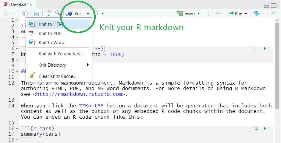
Knit the R markdown to HTML, PDF, and Word
2.9 Useful R Resources
You can find many useful resources (many of them are FREE) for learning R on the internet.
Free ebooks
bookdown is an R package that helps you to write and publish books using RStudio. Please check wonderful books on the site. You can freely read those books online.
In this site, you can find our textbook, R for Data Science (Hadley Wickham).
If you are interested in writing and publishing books on the internet like the ones on the bookdown website, please read bookdown: Authoring Books and Technical Documents with R Markdown (Yihui Xie). (This class will not cover this topic)
As you may already know, many researchers around the world create R packages and share with others through R package systems. If you are interested in creating your own R package, please read R Packages (Hadley Wickham). (This class will not cover this topic)
If you think you want to learn more advanced R at the end of this course, please read Advanced R (Hadley Wickham). (This class will not cover this topic)
If you prefer to read those books in Korean, try to translate books using the Chrome web browser: open the ebooks using Chrome web browser, click right mouse button, and choose “translate in Korean.”
You may already notice that the name “Hadley Wickham” appears here and there. Hadley Wickham contributes a lot to R community as a chief scientist at RStudio, creator of
tidyversepackage (ggplot2,dplyr,tidyr,stringr, etc.), and authors of many books. You can find more about Hadley in Hadley’s website.
RStudio Cheatsheets
One of the strengths of R is its package system. There are more than 18,000 packages that extend the functionality of base R. However, it’s difficult to remember all the details of such large number of packages.
RStudio provides RStudio Cheatsheets which summarize features of some important R packages in one or two pages. The cheatsheets will be nice references when you actually work with R for your own project.
2.10 Data Science Workflow
- The goal of this course is very simple. At the end of the course, each student is expected to have the ability to analyze her/his own data based on the following data science workflow presented by our textbook:
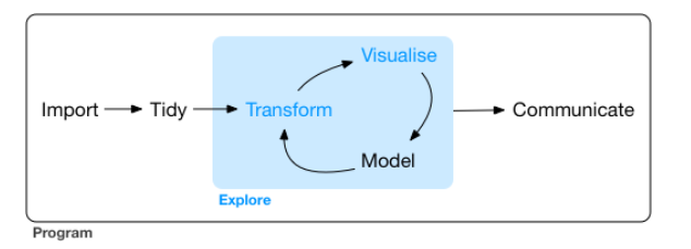
Typical Data Science Workflow
In Ch1 of R for Data Science, the author illustrates the process in typical data science project as follows
- import: read data into R from files (e.g., .csv, .xlsx)
- tidy, transform: get the original data into our desired form
- visualize: create plots to understand data or to present findings
- model: detect patterns from data
- communicate: tell your findings to others
2.10.1 Step0: Load all the packages you need for the analysis
2.10.2 Step1: Import your data
“First you must import your data into R. This typically means that you take data stored in a file, database, or web application programming interface (API), and load it into a data frame in R. If you can’t get your data into R, you can’t do data science on it!” (from RDS Ch1)
In this example, COVID19_Seoul.csv was obtained from Korean government’s data portal, data.go.kr and contains the information about the confirmed cases(확진자) in Seoul. I removed some variables and changed the variable names to English. The language of the website is Korean. If you want, you can use the translation option of your web browser (e.g., Google Chrome) to translate Korean to English.
In tidyverse, the readr package was developed to provide a fast and friendly way to read rectangular data (like csv, tsv, and fwf). Here is an overview and here is a cheatsheet.
Here are key functions in the readr package:
read_csv(): comma separated (CSV) filesread_tsv(): tab separated filesread_delim(): general delimited filesread_fwf(): fixed width filesread_table(): tabular files where columns are separated by white-space.read_log(): web log files
# Code Chunk 2-1
# read_csv() reads comma separated value (.csv) file
# read_csv() is a function in the readr package in tidyverse
# need to chagne the locale to read Korean character properly
covid19 <- read_csv("COVID19_Seoul.csv", locale = locale('ko', encoding = 'euc-kr'))
# Code Chunk 2-2
# data are stored as a tibble (data structure in tidyverse) named `covid19` in memory
# notice `date` is a date data type
covid19## # A tibble: 84,475 x 6
## id date region travel cause status
## <dbl> <date> <chr> <chr> <chr> <lgl>
## 1 84475 2021-09-08 구로구 <NA> 기타 확진자 접촉 NA
## 2 84474 2021-09-08 금천구 <NA> 감염경로 조사중 NA
## 3 84473 2021-09-08 송파구 <NA> 기타 확진자 접촉 NA
## 4 84472 2021-09-08 서초구 <NA> 기타 확진자 접촉 NA
## 5 84471 2021-09-08 구로구 <NA> 감염경로 조사중 NA
## 6 84470 2021-09-08 구로구 <NA> 감염경로 조사중 NA
## 7 84469 2021-09-08 강남구 <NA> 감염경로 조사중 NA
## 8 84468 2021-09-08 노원구 <NA> 기타 확진자 접촉 NA
## 9 84467 2021-09-08 강남구 <NA> 기타 확진자 접촉 NA
## 10 84466 2021-09-08 광진구 <NA> 감염경로 조사중 NA
## # ... with 84,465 more rows2.10.3 Step2: Tidy your data
“Once you’ve imported your data, it is a good idea to tidy it. Tidying your data means storing it in a consistent form that matches the semantics of the dataset with the way it is stored. In brief, when your data is tidy, each column is a variable, and each row is an observation. Tidy data is important because the consistent structure lets you focus your struggle on questions about the data, not fighting to get the data into the right form for different functions.” (from RDS Ch1)
covid19 is a tidy data and so we don’t need to tidy it. You may ask “Is there any column that is not a variable?”. Hadley says “yes”. You can consider a variable in the definition of the tidy data as the one that can be directly used in the later functions for a specific purpose. For example, we have the variable region in the covid19. Because of the region, we can easily calculate the number of confirmed cases by region by just using the variable region in the group_by() function.
In tidyverse, the tidyr package was developed to help you create tidy data. Here is an overview and here is a cheatsheet.
Here are key functions in the tidyr package:
pivot_longer(): lengthens data, increasing the number of rows and decreasing the number of columns (i.e., turning columns into rows)pivot_wider(): widens data, increasing the number of columns and decreasing the number of rows (i.e., turning rows into columns)separate(): separates a character column into multiple columns with a regular expression or numeric locationsunite(): unites multiple columns into one by pasting strings together
# Code Chunk 2-3
# `group_by()` is the key function in the `dplyr` package that allows us to apply functions by group.
# `summarise()` is the key function in the `dplyr` package that allows us to summarize variables.
# `%>%` is the pipe operator in the magrittr package that pipes (or connects) functions
# `covid19` is passed (or piped) into the `group_by()` function
# `n()` gives you the current group size
covid19 %>%
  group_by(region) %>%
  summarise(n = n())
## # A tibble: 27 x 2
## region n
## <chr> <int>
## 1 강남구 6123
## 2 강동구 3186
## 3 강북구 2185
## 4 강서구 3789
## 5 관악구 4712
## 6 광진구 2867
## 7 구로구 3154
## 8 금천구 1663
## 9 기타 2233
## 10 노원구 3389
## # ... with 17 more rows2.10.4 Step3: Transform your data
“Once you have tidy data, a common first step is to transform it. Transformation includes narrowing in on observations of interest (like all people in one city, or all data from the last year), creating new variables that are functions of existing variables (like computing speed from distance and time), and calculating a set of summary statistics (like counts or means). Together, tidying and transforming are called wrangling, because getting your data in a form that’s natural to work with often feels like a fight!” (from RDS Ch1)
When you import and tidy your data, it is rare that you get the data in the desired form you need for your data visualization and data modeling. So you need to further transform your data into the right form you need for your analysis.
In tidyverse, the dplyr package was developed to help you create tidy data. Here is an overview and here is a cheatsheet.
Here are key functions in the dplyr package:
mutate(): adds new variables that are functions of existing variablesselect(): picks variables based on their names.filter(): picks cases based on their values.summarise(): reduces multiple values down to a single summary.arrange(): changes the ordering of the rows.group_by(): performs operations by group.
# Code Chunk 2-4
# lubridate is the package for handling date and time
# `year()` in lubridate returns the year element of date
library(lubridate)
covid19 %>%
  mutate(year = year(date))  %>%    # mutate() creats a new variable
  filter(region %in% c("강남구", "강서구", "서대문구", "종로구"))  # filter() subsets rows
## # A tibble: 13,535 x 7
## id date region travel cause status year
## <dbl> <date> <chr> <chr> <chr> <lgl> <dbl>
## 1 84469 2021-09-08 강남구 <NA> 감염경로 조사중 NA 2021
## 2 84467 2021-09-08 강남구 <NA> 기타 확진자 접촉 NA 2021
## 3 84465 2021-09-08 서대문구 <NA> 감염경로 조사중 NA 2021
## 4 84419 2021-09-08 서대문구 <NA> 기타 확진자 접촉 NA 2021
## 5 84418 2021-09-08 종로구 <NA> 기타 확진자 접촉 NA 2021
## 6 84416 2021-09-08 종로구 <NA> 기타 확진자 접촉 NA 2021
## 7 84414 2021-09-08 종로구 <NA> 기타 확진자 접촉 NA 2021
## 8 84386 2021-09-08 강남구 <NA> 감염경로 조사중 NA 2021
## 9 84373 2021-09-08 종로구 <NA> 감염경로 조사중 NA 2021
## 10 84367 2021-09-08 강남구 <NA> 기타 확진자 접촉 NA 2021
## # ... with 13,525 more rows# Code Chunk 2-5
# lubridate is the package for handling date and time
library(lubridate)
covid19 %>%
mutate(year = year(date)) %>% # mutate() creates a new variable
filter(region %in% c("강남구", "강서구", "서대문구", "종로구")) %>%
group_by(region, year) %>% # group_by() performs operations by group
# Exercise: check what happens if you use `group_by(year, region)`
summarize(n = n()) # summarize() or summarise() summarize a variable## # A tibble: 8 x 3
## # Groups: region [4]
## region year n
## <chr> <dbl> <int>
## 1 강남구 2020 935
## 2 강남구 2021 5188
## 3 강서구 2020 1339
## 4 강서구 2021 2450
## 5 서대문구 2020 513
## 6 서대문구 2021 1801
## 7 종로구 2020 404
## 8 종로구 2021 9052.10.5 Step4: Visualize and Model your data
“Once you have tidy data with the variables you need, there are”“two main engines of knowledge generation”“: visualisation and modelling. These have complementary strengths and weaknesses so any real analysis will iterate between them many times.” (from RDS Ch1)
“Visualisation is a fundamentally human activity. A good visualisation will show you things that you did not expect, or raise new questions about the data. A good visualisation might also hint that you’re asking the wrong question, or you need to collect different data. Visualisations can surprise you, but don’t scale particularly well because they require a human to interpret them.”
“Models are complementary tools to visualisation. Once you have made your questions sufficiently precise, you can use a model to answer them. Models are a fundamentally mathematical or computational tool, so they generally scale well. Even when they don’t, it’s usually cheaper to buy more computers than it is to buy more brains! But every model makes assumptions, and by its very nature a model cannot question its own assumptions. That means a model cannot fundamentally surprise you.”
# Code Chunk 2-6
# `summarise()` is applied by group (date in this example)
covid19 %>%
  group_by(date) %>%
  summarise(n = n())
## # A tibble: 562 x 2
## date n
## <date> <int>
## 1 2020-01-24 1
## 2 2020-01-30 3
## 3 2020-01-31 3
## 4 2020-02-02 1
## 5 2020-02-05 2
## 6 2020-02-06 2
## 7 2020-02-16 2
## 8 2020-02-19 2
## 9 2020-02-20 5
## 10 2020-02-21 2
## # ... with 552 more rowsWhen you learn R, it is strongly recommended to follow the tidyverse style guide. R will understand your code anyway but using good coding style will increase the readability of your code. Remember the reader will be yourself in most of the case.
# Code Chunk 2-7
# the dataset created in Code Chunk 2-7 is passed (or piped) into `ggplot()`
covid19 %>%
  group_by(date) %>%
  summarise(n = n()) %>%
  ggplot(aes(x = date, y = n)) +
  geom_line()
# Code Chunk 2-8
# less readable code but same result
covid19 %>% group_by(date) %>% summarise(n = n()) %>%
ggplot(aes(x = date, y = n)) +
      geom_line()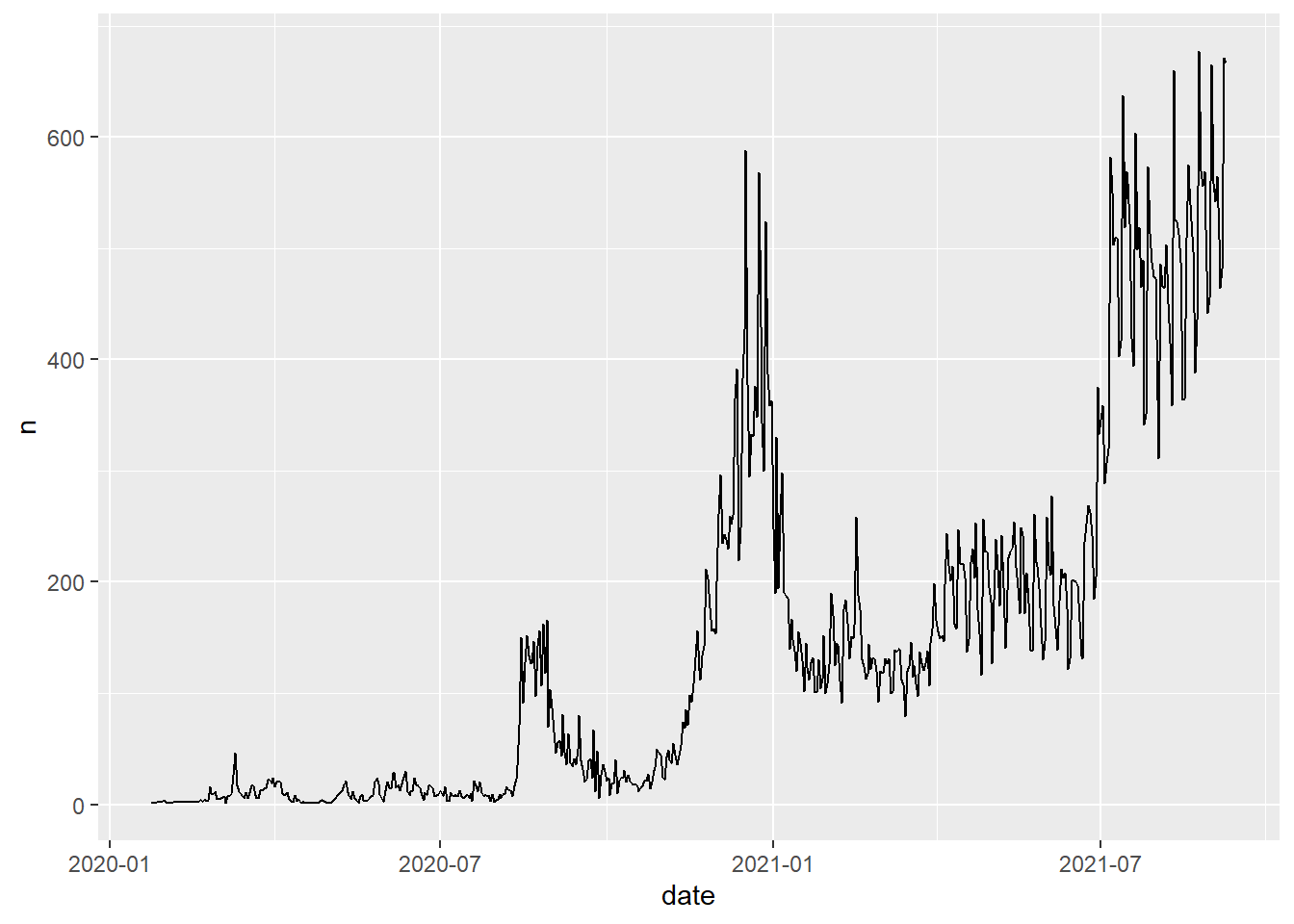
# Code Chunk 2-9
# `summarize()` is applied by `region` and `date`
covid19 %>%
  group_by(region, date) %>%
  summarise(n = n())
## # A tibble: 10,511 x 3
## # Groups: region [27]
## region date n
## <chr> <date> <int>
## 1 강남구 2020-02-26 2
## 2 강남구 2020-02-27 1
## 3 강남구 2020-02-28 3
## 4 강남구 2020-02-29 1
## 5 강남구 2020-03-01 1
## 6 강남구 2020-03-02 1
## 7 강남구 2020-03-05 1
## 8 강남구 2020-03-07 1
## 9 강남구 2020-03-08 1
## 10 강남구 2020-03-12 1
## # ... with 10,501 more rows# Code Chunk 2-10
# `color = region` is called a `aesthetic mapping` in ggplot2
# we have a separate line for each of four regions
# we are creating multiple subplots by subgroups in our data
covid19 %>%
filter(region %in% c("강남구", "강서구", "서대문구", "종로구")) %>% # select rows (or four regions)
group_by(region, date) %>%
summarise(n = n()) %>%
ggplot(aes(x = date, y = n, color = region)) +
geom_line() 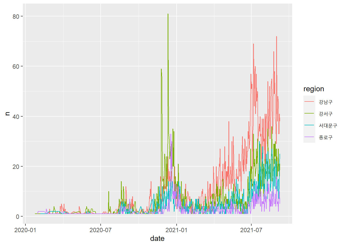
# Code Chunk 2-11
# Another way of creating subplots is to use `faceting`.
covid19 %>%
  filter(region %in% c("강남구", "강서구", "서대문구", "종로구")) %>%
  group_by(region, date) %>%
  summarise(n = n()) %>%
  ggplot(aes(x = date, y = n, color = region)) +
  geom_line() +
  facet_wrap(vars(region))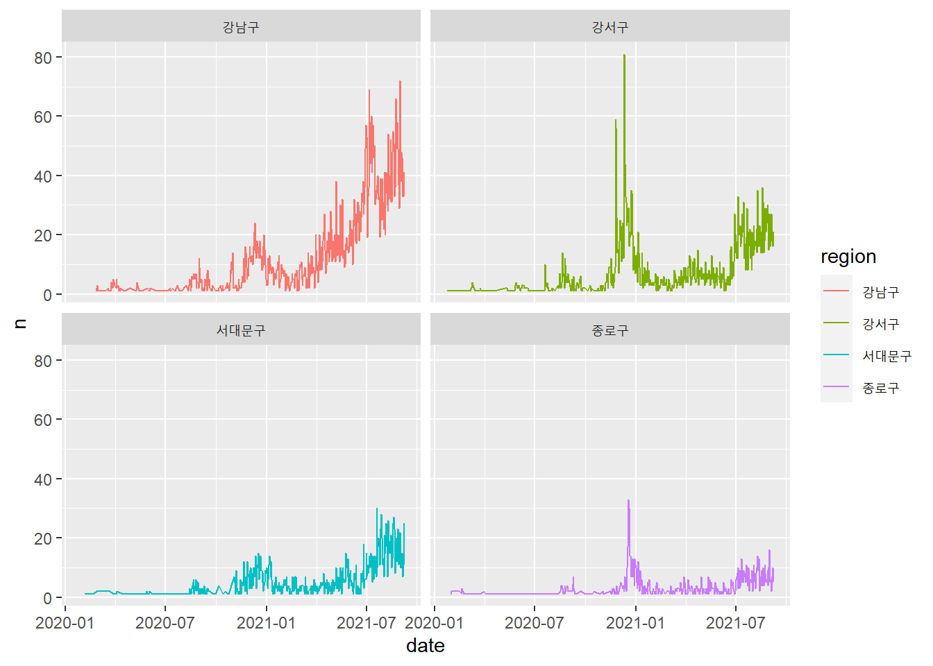
2.10.6 Step5: Communicate your findings
This lecture notes were created using the bookdown package (or Rmarkdown). This is an example of how you can communicate your findings with others. We will talk about the bookdown package next week. You will learn how to create your own bookdown like this lecture notes. I will upload the Rmarkdown file (.Rmd) in the cyber campus so that you can see how the Rmarkdown file can be translated into our lecture notes. In fact, the Rmarkdown file is a plain text file, which you can open with Notepad(메모장) in Windows or any text editor.
2.11 Quiz 2
For this quiz, we will use the built-in dataset in R, instead of actually importing the data from a file. We will use the iris data, a quite famous data in data science. The Iris data contains the length and the width of the sepals(꽃받침) and petals(꽃잎) in centimeters for 150 samples from three species (i.e., setosa, virginica, versicolor) of the Iris flower. You can google to find more information about the iris data such as this.
# Code Chunk 2-12
# head() is a function in base-R that display only the first 6 observations
head(iris)
## Sepal.Length Sepal.Width Petal.Length Petal.Width Species
## 1 5.1 3.5 1.4 0.2 setosa
## 2 4.9 3.0 1.4 0.2 setosa
## 3 4.7 3.2 1.3 0.2 setosa
## 4 4.6 3.1 1.5 0.2 setosa
## 5 5.0 3.6 1.4 0.2 setosa
## 6 5.4 3.9 1.7 0.4 setosaIs the iris tidy? No, the iris data is not a tidy dataset. Suppose that you want to calculate the mean of the petal(꽃잎) by species using the group_by() and summarize() functions in our previous examples. Can you do that? No you can’t do it easily because you don’t have a variable that contains sepal and petal as its values. The reason why we can’t easily calculate what we want is that the ’iris` is not tidy.
Now, I will tidy (or reshape)the original iris data using the functions in the tidyr package.
# Code Chunk 2-13
# tidying the raw data into the tidy data using `pivot_longer()` and `separate()` functions in the tidyr package
iris %>%
  pivot_longer(cols = -Species, names_to = "Part", values_to = "Value")
## # A tibble: 600 x 3
## Species Part Value
## <fct> <chr> <dbl>
## 1 setosa Sepal.Length 5.1
## 2 setosa Sepal.Width 3.5
## 3 setosa Petal.Length 1.4
## 4 setosa Petal.Width 0.2
## 5 setosa Sepal.Length 4.9
## 6 setosa Sepal.Width 3
## 7 setosa Petal.Length 1.4
## 8 setosa Petal.Width 0.2
## 9 setosa Sepal.Length 4.7
## 10 setosa Sepal.Width 3.2
## # ... with 590 more rows# Code Chunk 2-14
# tidying the raw data into the tidy data using `pivot_longer()` and `separate()` functions in the tidyr package
iris %>%
pivot_longer(cols = -Species, names_to = "Part", values_to = "Value") %>%
separate(col = "Part", into = c("Part", "Measure"))## # A tibble: 600 x 4
## Species Part Measure Value
## <fct> <chr> <chr> <dbl>
## 1 setosa Sepal Length 5.1
## 2 setosa Sepal Width 3.5
## 3 setosa Petal Length 1.4
## 4 setosa Petal Width 0.2
## 5 setosa Sepal Length 4.9
## 6 setosa Sepal Width 3
## 7 setosa Petal Length 1.4
## 8 setosa Petal Width 0.2
## 9 setosa Sepal Length 4.7
## 10 setosa Sepal Width 3.2
## # ... with 590 more rowsNow, the dataset created by the code chunk 2-14 is a tidy dataset because each column is a variable that we can use in our later functions. The benefits of the tidy data become clear. With tidy datasets, you can easily transform and visualize your data. For example, you can eaily calculate the mean of Value by Species.
# Code Chunk 2-14
# tidying the raw data into the tidy data using `pivot_longer()` and `separate()` functions in the tidyr package
iris %>%
  pivot_longer(cols = -Species, names_to = "Part", values_to = "Value") %>%
separate(col = "Part", into = c("Part", "Measure")) %>%
group_by(Species) %>%
summarise(m = mean(Value, na.rm = TRUE))## # A tibble: 3 x 2
## Species m
## <fct> <dbl>
## 1 setosa 2.54
## 2 versicolor 3.57
## 3 virginica 4.28So here are your quiz problems for week2. You need to use some summary functions for descriptive statistics in Week 1 lecture notes.
Quiz 2-1: What is the standard deviation of the
Valueforsetosa?Quiz 2-2: What is the median of the
Valueforversicolor?Quiz 2-3: What is the mean of the
ValueforPetalinsetosa?Quiz 2-4: What is the mean of the
ValueforWidthofPetalinversicolor?