Chapter 1 Introduction to data analysis

1.1 Welcome to the Course!

Hi everyone, welcome to the course. This is the introduction to R course at Ewha Womans University.
R is a great programming language for statistical analysis and data science. I hope you enjoy R in this course and find many useful applications for your own field.
This course is designed for students who don’t have any programming background in social science.
In this lecture note, this font represents R commands, variable names, and package names.
In order to maximize your learning in this semester, you should read the weekly reading assignment in our textbook, R for Data Science.
If you have any question on this lecture (e.g., errors in running R, questions about quiz), please send your questions to r.ewha.questions.2021@gmail.com. Then, Iand TA(Teaching Assistant) will answer your questions.
In this lecture notes, I will include interactive code chunks provided by DataCamp that will allow you to actually run and practice R codes within this lecture notes. Please type 3+4 and click Run button to ask R to calculate the expression.

eyJsYW5ndWFnZSI6InIiLCJzYW1wbGUiOiIjIFRoaXMgaXMgdGhlIGludGVyYWN0aXZlIGNvZGUgY2h1bmsuIFxuIyBQbGVhc2UgdHlwZSBgMys0YCBhbmQgY2xpY2sgYFJ1bmAgYnV0dG9uIGJlbG93IHRvIGdldCB0aGUgcmVzdWx0In0=

1.2 Types of Data Analysis

Before talking about R and social problems, let’s talk about the types of data analysis first.
Leek & Peng(2015) categorized data analysis into the 6 types as presented in the table below, and emphasized “mistaking the type of question being considered is the most common error in data analysis.”

Types of Data Analysis	Questions being asked
Descriptive data analysis(기술통계분석)	seek to summarize(요약) the measurement in a single data set without further interpretation(e.g., US Census)
Exploratory data analysis(탐색적자료분석)	search for discoveries(발견), trends, correlations, or relationships between the measurements to generate ideas or hypotheses(e.g., The four-star planetary system Tatooine)
Inferential data analysis(추론분석)	quantify whether an observed pattern will likely hold beyond the data set in hand or in population(모집단)(e.g., a study of whether air pollution correlates with life expectancy in US)
Predictive data analysis(예측분석)	predict(예측) another measurement (the outcome) on a single person or unit(e.g., prediction of how people will vote in an election)
Causal data analysis(인과관계분석)	seek to find out what happens to one measurement on average if you make another measurement change(인과, e.g., causal relationship between smoking and cancer)
Mechanistic data analysis(결정론적관계분석)	seek to show that changing one measurement always and exclusively leads to a specific, deterministic behavior in another(인과, e.g., wing design)

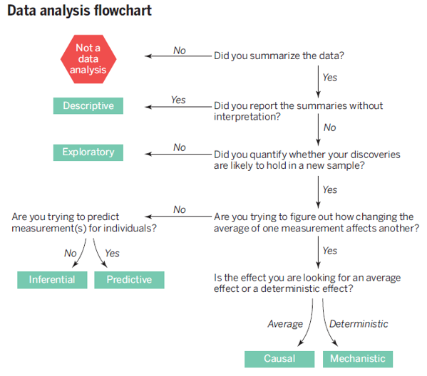
from Leek & Peng (2015)

Leek & Peng(2015)’s main point is that we should keep in mind the type of question being asked by our own data analysis. In other words, we should say what we can say, not what we want to say.
Leek & Peng(2015) presents a table showing common mistakes

Real Question Type	Perceived Question Type	Phrase Describing Error
Inferential	Causal	Correlation does not imply causation
Exploratory	Inferential	Data Dredging (or p-hacking)
Exploratory	Predictive	Overfitting(과적합)
Descriptive	Inferential	n of 1 analysis

Leek & Peng(2015) mentioned a very important statement that we should keep in mind when we use data science to solve social problems:

“In nonrandomized experiments, it is usually only possible to determine the existence of a relationship between two measurements, but not the underlying mechanism or the reason for it.”

It is known that the best way to investigate causal relationship is to conduct randomized experiments. However, unlike in natural science, it is not easy to conduct randomized experiments in social science because of ethical and practical reasons. The fundamental dilemma of data analysis in social science is that we essentially want to make causal statements in the absence of randomized experiments. Many statistical tools we use are just correlational.
In the field of the philosophy of science, it is usually said that the goals of science is explanation and prediction:

“Historically, social scientists have sought out explanations of human and social phenomena that provide interpretable causal mechanisms, while often ignoring their predictive accuracy. We argue that the increasingly computational nature of social science is beginning to reverse this traditional bias against prediction.” (Hofman et al., 2017)

1.3 Causality

Then, what is causality(인과관계)?
- According to Cohen et al.(2014), X is a cause of Y if
  - X precedes Y in time (temporal precedence, 시간의 우선성).
  - Some mechanism whereby this causal effect operates can be posited (causal mechanism, 인과기제)
  - A change in the value of X is accompanied by a change in the value of Y on the average (association or correlation, 상관관계)
  - The effects of X on Y can be isolated from the effects of other potential variables on Y (non-spuriousness or lack of confounders, 다른 대안적 설명의 배제)
- According to Bollen(1989), the conditions for causal inference are
  - For X to cause Y, X must precede Y in time (temporal order)
  - For X to cause Y, Y should be isolated from all other influences except X (isolation)
  - For X to cause Y, X and Y must be correlated (association)
Correlation is a necessary condition(필요조건) for causality, not a sufficient condition(충분조건). In order words, correlation does not imply causality(상관관계는 인과관계를 함축하지 않는다).

A randomized experiment is defined by the following three conditions:
- Random assignment of subjects to groups(실험대상의 무작위 할당)
  - Each subject have equal probability to be assigned to experimental and control groups.
- Manipulation of an independent variable(독립변수의 조작)
  - Researcher can give treatments(처치) or interventions(개입) to an experimental group.
- Control of extraneous variables(외생변수의 통제)
  - Researcher can control variables other than the independent variable that can influence the outcome.
A randomized experiment allows us to talk about causality because it effectively eliminates alternative explanations and attributes the changes in the outcome solely to the changes in the independent variable(무작위 실험은 다른 대안적 설명을 배제하고 결과값의 차이를 유일하게 종속변수의 차이로 설명한다).
Research can be categorized into experimental(실험연구) and non-experimental studies(비실험연구). In social science, most research are non-experimental, which makes it difficult for us to talk about causality.

1.4 Correlation

Covariance(공분산) between two variables, $Cov(X, Y)$, measures the strength and direction of the linear relationship between two variables:

\[Cov(X,Y) = E[(X-\mu_x)(Y-\mu_y)]\]

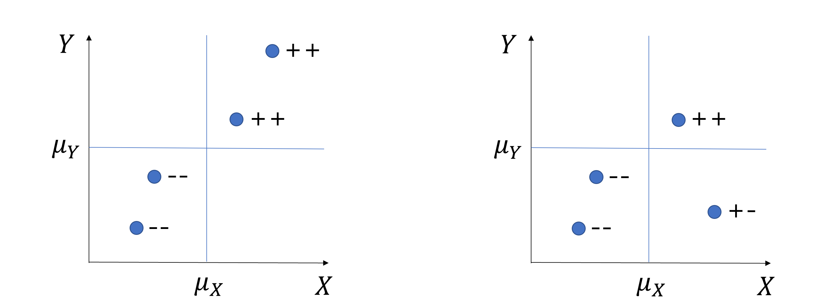
High covariance vs Low covariance

Because covariance depend on the scale of variables, we need a standardized version of covariance, a correlation coefficient(상관계수):

\[\rho(X, Y) = \frac{Cov(X,Y)}{\sigma_X\sigma_Y}, \text{where } \sigma \text{=standard deviation(표준편차)}\]

Correlation coefficients have values between -1 and 1 (i.e., $-1\le\rho\le1$) and the values close to -1 or 1 indicate strong linear relationship.

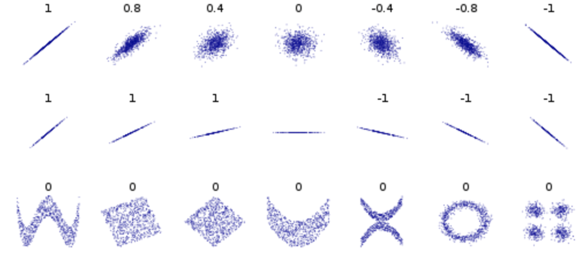
Correlation coefficients (from wiki)

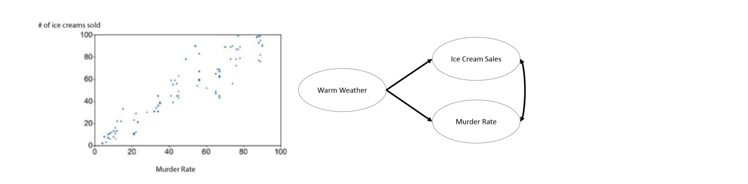
Again, correlation does not imply causality. Here are some fun examples of correlated variables: Spurious correlations
So, what can we do to talk about causality when we cannot conduct randomized experiment in social science?

“In many scientific fields, and especially the social sciences, statistical methods are used nearly exclusively for testing causal theory. Given a causal theoretical model, statistical models are applied to data in order to test causal hypotheses. In such models, a set of underlying factors that are measured by variables X are assumed to cause an underlying effect, measured by variable Y . Based on collaborative work with social scientists and economists, on an examination of some of their literature, and on conversations with a diverse group of researchers, I conjecture that, whether statisticians like it or not, the type of statistical models used for testing causal hypotheses in the social sciences are almost always association-based models applied to observational data. Regression models are the most common example. The justification for this practice is that the theory itself provides the causality. In other words, the role of the theory is very strong and the reliance on data and statistical modeling are strictly through the lens of the theoretical model. The theory–data relationship varies in different fields.While the social sciences are very theory-heavy, in areas such as bioinformatics and natural language processing the emphasis on a causal theory is much weaker.” (Shmueli, 2010))

1.5 Descriptive Data Analysis

The goal of descriptive data analysis is to summarize measurements.
R provide many summary functions for descriptive statistics
- Measures of central tendency(중심위치의 척도)
  - mean() for mean
  - median() for median
- Measures of dispersion(산포정도의 척도)
  - IQR() for inter-quartile range
  - mad() for median absolute deviation
  - sd() for standard deviation
  - var() for variance
- Measures of position or order(위치의 척도)
  - quantile() for nth quantile
  - min() for minimum value
  - max() for maximum value
- Various descriptive statistics
  - summary() in Base-R
  - describe() in the psych package
R comes with many built-in datasets which are useful for our practice. You can check the list here.

# the data `cars` give the speed of cars and the distances taken to stop
# type '?cars` in your R console to see the help documents. 
# head() display only first few observations
head(cars)

##   speed dist
## 1     4    2
## 2     4   10
## 3     7    4
## 4     7   22
## 5     8   16
## 6     9   10

The mean of the variable speed can be obtained as follows:

# na.rm = TRUE: NA(missing value) will be removed when calculating the mean
# cars$speed: $ is used to access a variable in a dataframe
mean(cars$speed, na.rm = TRUE)

## [1] 15.4

Sometimes we want to get various summary statistics for all variables within a dataset.

# summary() function belongs to Base-R. So, we don't need any additional package. 
# In R, a package is a collection of functions designed for a specific purpose. 
summary(cars)

##      speed           dist       
##  Min.   : 4.0   Min.   :  2.00  
##  1st Qu.:12.0   1st Qu.: 26.00  
##  Median :15.0   Median : 36.00  
##  Mean   :15.4   Mean   : 42.98  
##  3rd Qu.:19.0   3rd Qu.: 56.00  
##  Max.   :25.0   Max.   :120.00

# In R, "package_name::function_name" is used when we call a function within a package. 
# With "psych::describe()", we are calling the describe() function within the psych package. 
psych::describe(cars)

##       vars  n  mean    sd median trimmed   mad min max range  skew kurtosis
## speed    1 50 15.40  5.29     15   15.47  5.93   4  25    21 -0.11    -0.67
## dist     2 50 42.98 25.77     36   40.88 23.72   2 120   118  0.76     0.12
##         se
## speed 0.75
## dist  3.64

Exercise 1-1. Calculate descriptive statistics for cars$speed using all the R summary functions for descriptive statistics presented above. You can compare your own results with the numbers in the table produced by psych::describe(cars).

eyJsYW5ndWFnZSI6InIiLCJzYW1wbGUiOiIjIFRoaXMgaXMgdGhlIGludGVyYWN0aXZlIGNvZGUgY2h1bmsgcHJvdmlkZWQgYnkgRGF0YUNhbXAifQ==

1.6 Exploratory Data Analysis

The goal of exploratory data analysis is to discover patterns among measurements.

“This book is about exploratory data analysis, about looking at data to see what it seems to say. It concentrates on simple arithmetic and easy-to-draw pictures. It regards whatever appearances we have recognized as partial descriptions, and tries to look beneath them for new insights. Its concern is with appearance, not with confirmation.” (Tukey, 1977)

# library(ggplot2) loads ggplot2 package into your computer's memory
# You need to load any R package into your memory before you use it
# ggplot2 package is the R package for data visualization 
# The code below creates a scatter plot between speed and distance
# We will talk about ggplot2 later 
# Can you find any pattern of relationship between speed and distance? 
library(ggplot2)

## Warning: package 'ggplot2' was built under R version 4.0.5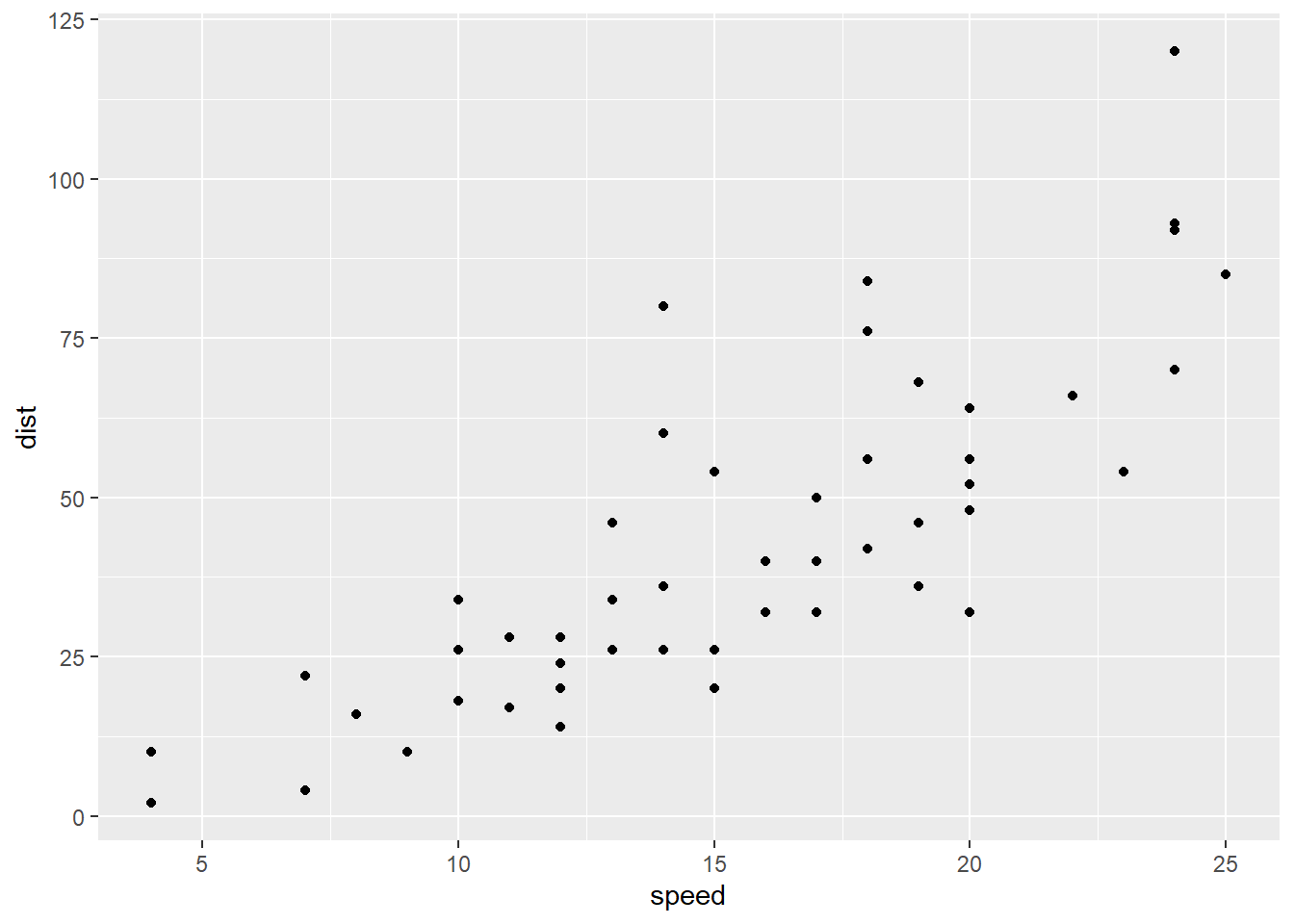

ggplot(data = cars, aes(x = speed, y = dist)) + 
    geom_point()

Exercise 1-2. Your first(?) ggplot2 plot. Please replicate the scatter plot above.

eyJsYW5ndWFnZSI6InIiLCJzYW1wbGUiOiIjIFBsZWFzZSByZXBsaWNhdGUgdGhlIHNjYXR0ZXIgcGxvdCBhYm92ZSJ9

1.7 Inferential Data Analysis

The goal of inferential data analysis is to quantify whether an observed pattern will likely hold beyond the data set in hand or in population.
In other words, we want to talk about
- what we don’t know based on what we know
- population based on samples
- the whole based on the part
As an example of inferential data analysis, let’s fit a regression model to cars data to make inference about the relationship between speed and distance in population.

# lm() fits a regression model to your data
# In this example, `dist` is a dependent variable, and `speed` is an independent variable
fit <- lm(dist ~ speed, data = cars)
summary(fit)

## 
## Call:
## lm(formula = dist ~ speed, data = cars)
## 
## Residuals:
##     Min      1Q  Median      3Q     Max 
## -29.069  -9.525  -2.272   9.215  43.201 
## 
## Coefficients:
##             Estimate Std. Error t value Pr(>|t|)    
## (Intercept) -17.5791     6.7584  -2.601   0.0123 *  
## speed         3.9324     0.4155   9.464 1.49e-12 ***
## ---
## Signif. codes:  0 '***' 0.001 '**' 0.01 '*' 0.05 '.' 0.1 ' ' 1
## 
## Residual standard error: 15.38 on 48 degrees of freedom
## Multiple R-squared:  0.6511,	Adjusted R-squared:  0.6438 
## F-statistic: 89.57 on 1 and 48 DF,  p-value: 1.49e-12

Here are the definitions of some basic terminologies in inference

Term	Definition
Population(모집단)	The entire set of subjects we are interested in
Parameter(모수)	A numerical characteristics of a population
Estimate(추정값)	Our best guess about the population parameters that are calculated based on our samples. It is very important to keep in mind that the values of the estimate vary across different samples. This is called the sampling variability.
Sampling distribution(표본분포)	The distribution of the values of an estimate (or statistic) across infinite number of different samples.
Standard error(표준오차)	The measure of the sampling variability of an estimate measured by the standard deviation of the sampling distribution. Standard error can be considered as the measure of accuracy of an estimate.
t value(t값)	A statistic to test the null hypothesis $H_0: \beta=0$
p-value(유의확률)	Given the assumption that the null hypothesis is true, a probability of getting a test statistic as extreme or more extreme than the calculated test statistic. $p<0.05$ is considered as the evidence that the null hypothesis is not consistent with data. That is, if $p<0.05$, we will reject $H_0$.

Based on the regression result above, we can conclude that the speed of a car significantly predicted the distances taken to stop, $\beta = 3.9324, p < 0.01$. We can use the term significantly because our $p<0.05$, indicating we reject $H_0: \beta=0$.
You can add a regression line to the scatter plot.

# geom_smooth() adds a regression line to the scatter plot
library(ggplot2)
ggplot(data = cars, aes(x = speed, y = dist)) + 
    geom_point() +
    geom_smooth(method = "lm")

## `geom_smooth()` using formula 'y ~ x'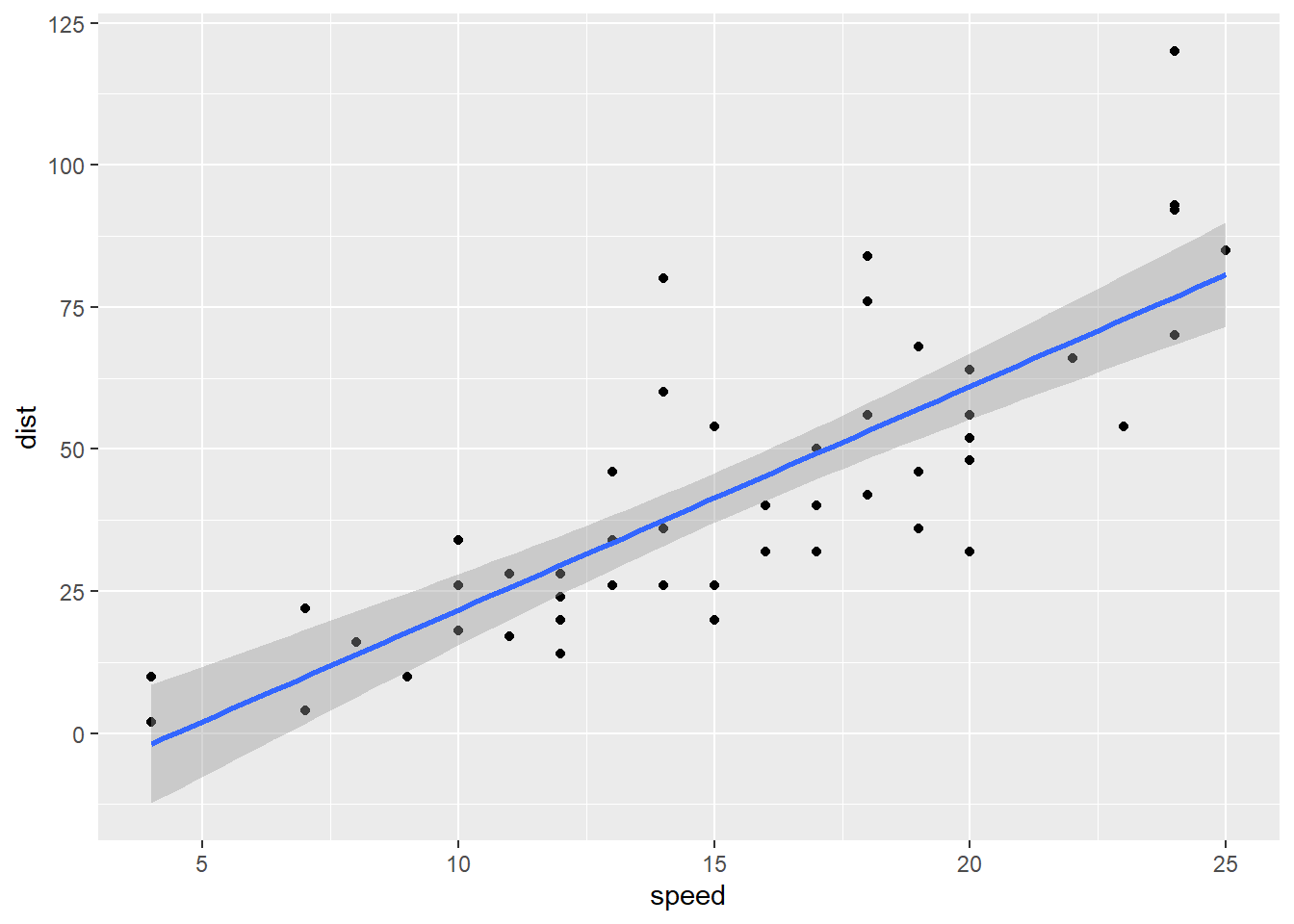

Exercise 1-3. Please replicate the regression results and scatter plot with regression line above.

eyJsYW5ndWFnZSI6InIiLCJzYW1wbGUiOiIjIFBsZWFzZSByZXBsaWNhdGUgdGhlIHJlZ3Jlc3Npb24gcmVzdWx0cyBhbmQgc2NhdHRlciBwbG90IHdpdGggcmVncmVzc2lvbiBsaW5lIGFib3ZlIn0=

1.8 Predictive Data Analysis

The goal of predictive data analysis is to predict the outcome of an individual.
Machine learning is a sub-field of an artificial intelligence which focuses on learning patterns from data to improve the performance of a specific task. Machine learning can be categorized into supervised learning, unsupervised learning, and reinforcement learning. The supervised learning has been widely used for predictive data analysis.
The key for accurate prediction is to learn from data only the generalizable relationship that are valid for previously unseen data.
In R, the carat package has been widely used to build predictive models. We will talk about predictive data analysis using the carat package later.
If you are interested in predictive data analysis, you can start to read the following readings:
- For theoretical understanding about predictive data analysis using supervised learning, please read Yarkoni & Westfall (2017)
- For carat package usage, please check Kuhn’s(the author of the carat package) manual here
- For a short version of carat manual, please read Kuhn(2008)

1.9 R vs RStudio

What is R? R is a programming language. What is a programming language? A programming language is a formal language consisting of a set of instructions (or commands) that allow us to make computers work for us. For example, when you execute the following R commands, there should be something in your computer that can understand the set of instructions (or commands) and then create a plot for you. That’s R. So we need to install R to learn R programming language.

# geom_smooth() adds a regression line to the scatter plot
library(ggplot2)
ggplot(data = cars, aes(x = speed, y = dist)) + 
    geom_point() +
    geom_smooth(method = "lm")

## `geom_smooth()` using formula 'y ~ x'

Then, what is a RStudio? As the first line of the R project website(https://www.r-project.org/) says, “R is a free software environment for statistical computing and graphics.”, meaning that the R provides some features (e.g., source editor for editing our R codes) that can help R programming. But it’s not that convenient :(
RStudio is an convenient interface between R and users. It is an integrated development environment (IDE) for R.
So, the best practice of using R is to install both R and RStudio, and then use RStudio for your programming. Note that R is still a workhorse and RStudio is an interface for R.

1.9.1 Let’s Install R to your local computer

Please install R for your own operating system from https://www.r-project.org/

Click the download R link

Click any mirror server you like (e.g., 0-Cloud)

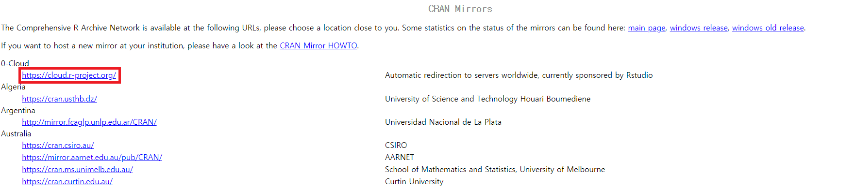
Mirrors

Click the operating system in your computer

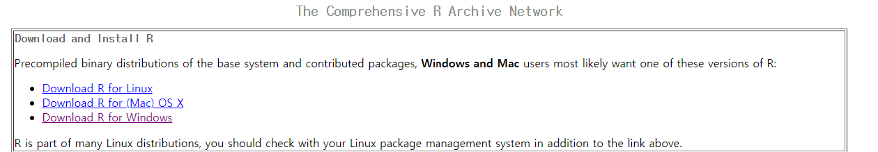
Click the base button

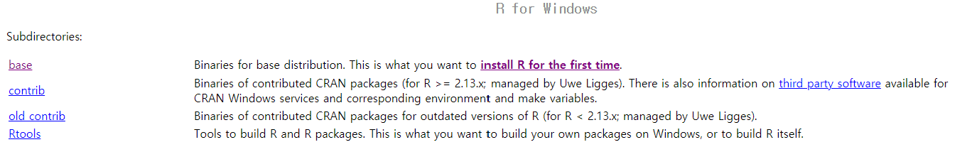
Click the Download R button

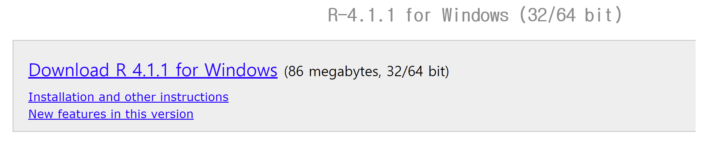
Click the downloaded file to start your installing process

(You will find lots of videos demonstrating installing process on YouTube)

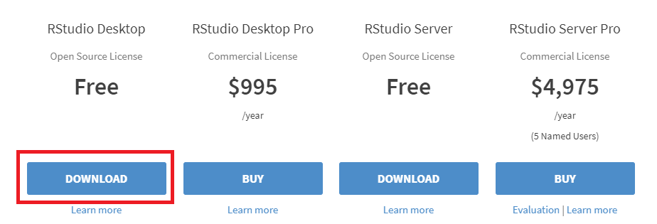
1.9.2 Let’s install RStudio to your local computer

Please install FREE version of RStudio Desktop for your own operating system from https://rstudio.com/products/rstudio/download/.

This is the special instruction only for students who are using Korean version of Windows. Those students who are using English version of Windows can ignore this instructions.

한글 윈도우쓰시는 한국 학생들은 RStudio 설치시 다음과 같은 경우에 RStudio가 설치가 안돼거나 설치되어도 작동이 안할 수 있습니다.
- 사용자명이 한글로 되어 있는경우
- 컴퓨터 이름이 한글로 되어 있는경우
- 설치 폴더 경로중에 한글이 포함된 경우
한글 윈도우를 쓰시는 학생들은 사용자명, 컴퓨터 이름, 설치 폴더 경로가 모두 영어가 되어 있는지를 확인하고 다음 링크의 지시를 따라서 설치를 진행해 주시기 바랍니다: https://chancoding.tistory.com/16
구글이나 네이버가 가셔서 “RStudio 한글 설치” 이런정도의 키워드로 검색을 해보시면 RStudio설치시 한글과의 충돌로 인한 문제점에 대한 많은 문서들을 발견할 수 있습니다. 문제가 생기면 우선 구글이나 네이버 검색을 통해서 해결해 보시기 바랍니다. 수강인원이 200명이 넘는 대형강의이기 때문에 조교 선생님들이나 제가 최선을 다해서 도와드리겠지만, 하나하나 수강생들의 특수한 경우에 모두 해결책을 제시해 드리기 힘든점 양해 부탁드립니다.

1.10 References

Cohen, P., West, S. G., & Aiken, L. S. (2014). Applied multiple regression/correlation analysis for the behavioral sciences. Psychology press.
Bollen, K. A. (1989). Structural equations with latent variables (Vol. 210). John Wiley & Sons.
Hofman, J. M., Sharma, A., & Watts, D. J. (2017). Prediction and explanation in social systems. Science, 355(6324), 486-488.
Kuhn, M. (2008). Building predictive models in R using the caret package. Journal of statistical software, 28(1), 1-26.
Leek, J. T., & Peng, R. D. (2015). What is the question?. Science, 347(6228), 1314-1315.
Shmueli, G. (2010). To explain or to predict?. Statistical science, 25(3), 289-310.
Tukey, J. W. (1977). Exploratory data analysis (Vol. 2, pp. 131-160).
Yarkoni, T., & Westfall, J. (2017). Choosing prediction over explanation in psychology: Lessons from machine learning. Perspectives on Psychological Science, 12(6), 1100-1122.

R @ Ewha (Sunbok Lee)