Chapter 6 Visualization
In this chapter, we will use R for visualizing data. Along with descriptives, any analyst needs to be able to present data visually. R has some basic built in functions for graphics. However, this chapter examines the use of a specific package for visualization as it is both powerful and is used by more advanced users as well. Thus, it allows for more sophisticated visualization as one progresses.
Very often, it is common to look at bar charts to examine data. The package we will use to create visualizations is ggplot2. Ggplot2 allows for visualization using layers and addition of different commands that are useful in continuing to build and modify a visual representation. In addition, it can be easily re-used with slight modification for different variables. In the section below, we will examine the variable gender visually.
6.1 Visualization of Single Variables
The typical syntax for creating a visualization specifies the dataset to be used, aesthetics of mapping that specifies the variable, and the type of chart such as barchart or a scatterplot etc to be used. These can be enhanced further by adding additional syntax for title, color, and other such aesthetic elements. For example, a barchart for gender is created as follows:
6.1.1 Bar Chart with No Formatting
##We are using dataframe df to plot Gender on x axis, y axis by default is count, and we specify that we would like a bar chart
ggplot(df,mapping=aes(x=as.factor(gender)))+geom_bar()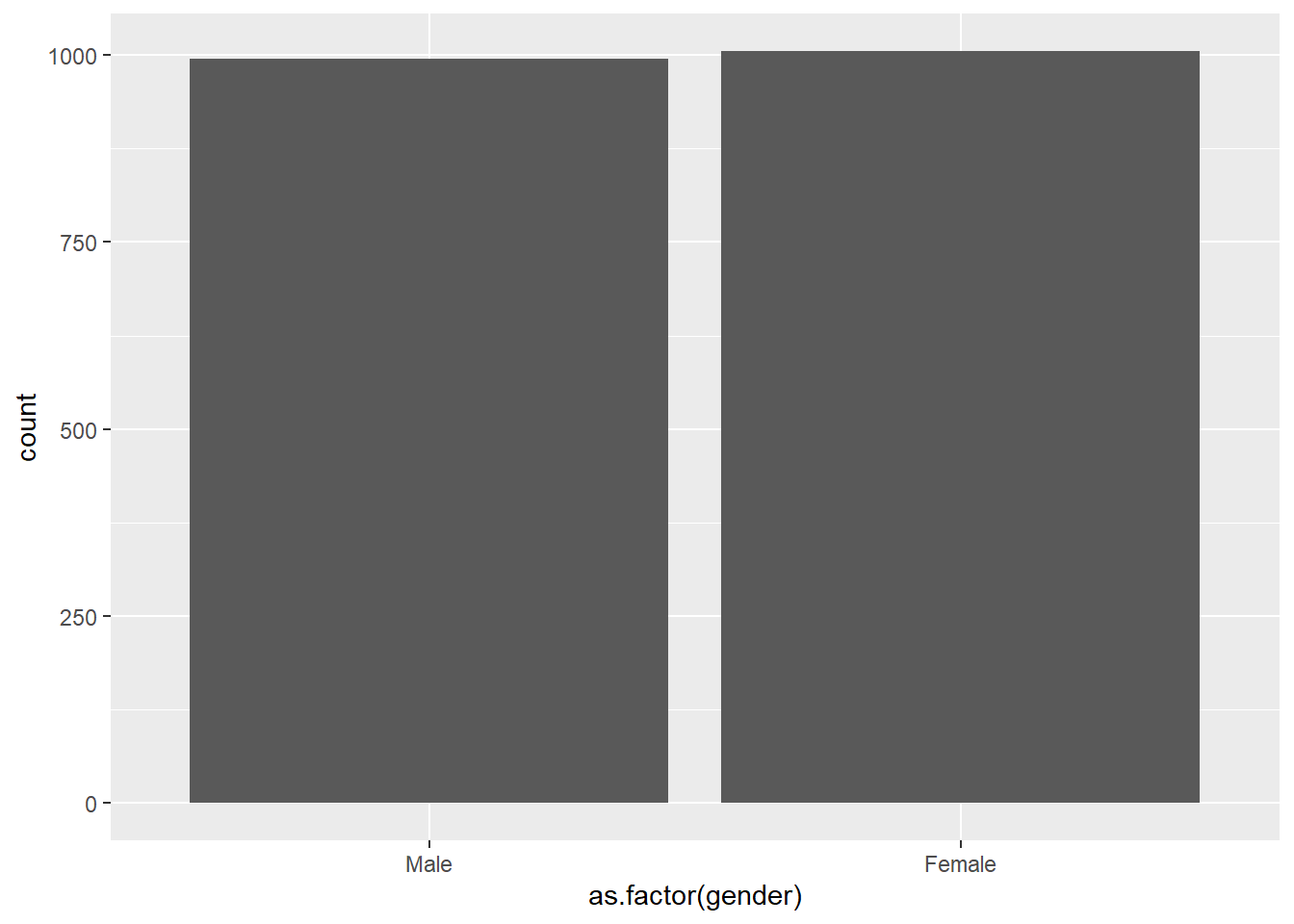
Figure 6.1: Bar Chart with No Formatting
6.1.2 Bar Chart with Formatting
The above chart is not very pleasing. We can make a few changes by adding a title, labels, and color to the chart as follows.

Figure 6.2: Bar Chart with Formatting
6.1.3 Horizontal Bar Chart
If we wanted the plot to appear horizontally, we simply need to change the aes mapping to y instead of x as follows:
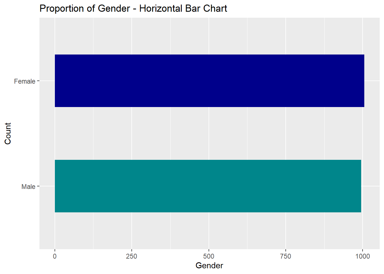
Figure 6.3: Hoizontal Bar Chart with Formatting
As seen in the chart, we would like to improve upon it by adding labels to see the actual count of cases or any other statistics that we are plotting which we can do using geom_text. However, it is easiest to do this in one of two ways. The simplest way is to use the package dplyr, to manipulate the data to be in a form that can be plotted easily. Although, dplyr is quite powerful, here we will only look at a few uses. The package works similar to how we used piping earlier. In order to get counts as values on the chart, it is helpful to simply have a dataframe of gender with type and count as variables as follows:
##   gender    n
## 1      1  995
## 2      2 1005
6.1.4 Creating Labels for Charts
As seen above, we now have a new dataframe with just the variables of interest in plotting, making it easy to specify labels as follows using an additional command of geom_text:
# Use data count_data
# map x as gender and y as n
# create a bar chart with values of the variable in dataframe using "identity" -- this is important
# use n as label specified in geom_text
ggplot(count_data,mapping=aes(x=as.factor(gender),y=n))+geom_bar(stat="identity",fill=c("turquoise4","blue4"),width=0.4)+ggtitle("Proportion of Gender")+xlab("Gender")+ylab("Count")+geom_text(aes(label=n),color="black",size=3)
Figure 6.4: Bar Chart with Variables in New Data Frame
6.1.5 Creating Chart with Percentages
By simply creating a new dataframe with the variables and values of interest, plotting is made much easier and more visually appealing. For example, we can use dplyr again to create a new dataframe that has percentages as follows:
##   gender    n percent
## 1      1  995   49.75
## 2      2 1005   50.25
As seen above, we now have a dataframe with three variables. The command mutate defines a new variable using existing variable n in the new dataframe count(gender). Now we can use this new dataframe which readily has percentages available to create a chart that shows percentages following the same method as before with change in specified variable names.
# Use data count_data
# map x as gender and y as percentage
# create a bar chart with values of the variable in dataframe using "identity" -- this is important
# use percent as label specified in geom_text
ggplot(percent_data,mapping=aes(x=as.factor(gender),y=percent))+geom_bar(stat="identity",fill=c("turquoise4","blue4"),width=0.45)+ggtitle("Proportion of Gender")+xlab("Gender")+ylab("Percentage")+geom_text(aes(label=percent),color="black",size=3)
Figure 6.5: Bar Chart with Percentages
6.1.6 Positioning of Values in Chart
We can modify the above commands with vjust, hjust, and size to change the size and position of values on the chart as follows:
# Use data count_data
# map x as gender and y as percentage
# create a bar chart with values of the variable in dataframe using "identity" -- this is important
# use percent as label specified in geom_text
ggplot(percent_data,mapping=aes(x=as.factor(gender),y=percent))+geom_bar(stat="identity",fill=c("turquoise4","blue4"),width=0.45)+ggtitle("Proportion of Gender")+xlab("Gender")+ylab("Percentage")+geom_text(aes(label=percent),color="maroon",size=5,vjust=-.25)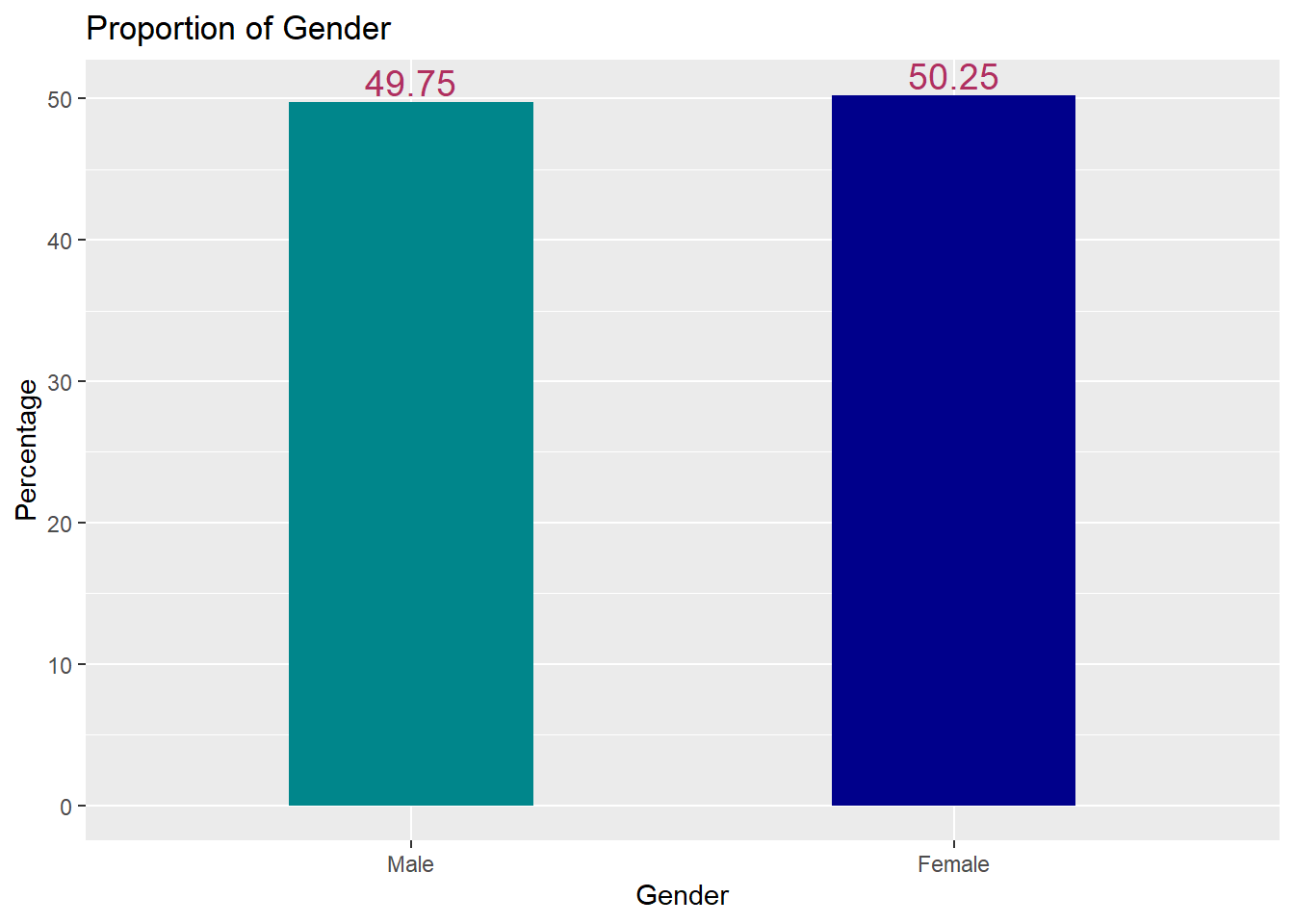
Figure 6.6: Bar Chart with Percentages Resized
Since the numbers above the chart are not clearly visible due to the scale of Y axis, it is possible to rescale as follows for better visibility:
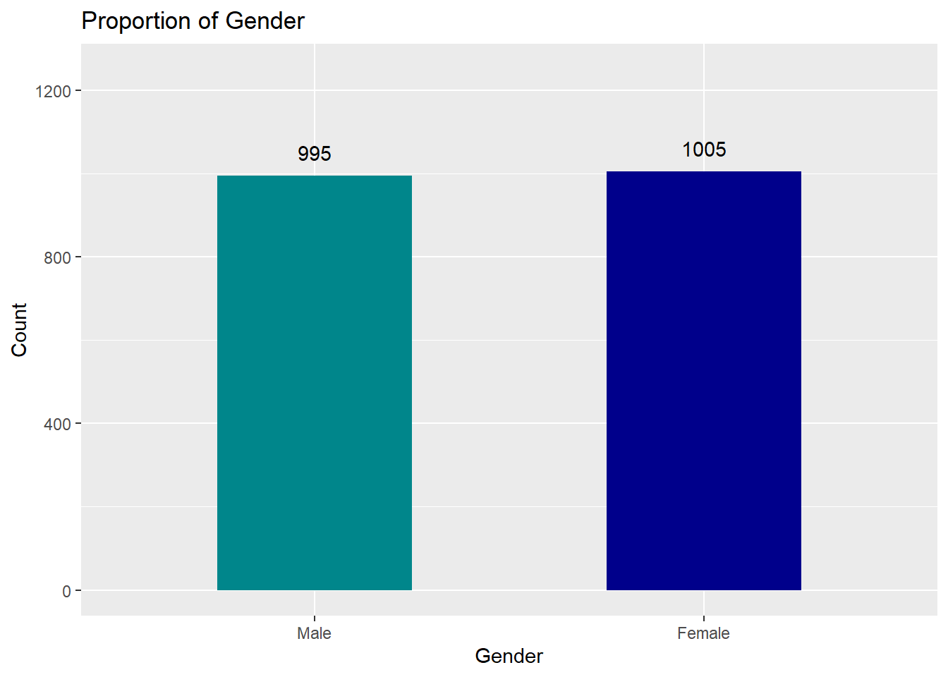
Figure 6.7: Bar Chart with Counts with Rescaled Y axis
The above code adjusts for positioning of the numbers vertically slightly above the bar and the ylim command allows us to adjust the y scale so the numbers are more visible on the plot. Similarly, it is possible to use xlim to adjust the scale for X-axis.
The package ggplot offers many options in types of charts such as geom_point for scatterplots, geom_density for density plots etc. It also offers many options in use of colors to make charts visually appealing, precisely 657 different colors with many different shades within one specific color. Following is a sample list of some colors that you have available for use in R.
"white" "aliceblue" "aquamarine" "aquamarine1" "aquamarine2" "blue" "cadetblue" "coral" "darkblue" "green" "gray" "lightblue" "hotpink" "magenta" "maroon" "navy" "orange" "palegreen" "pink" "purple" "red" "sienna" "tan" "violet" "yellow"
6.2 Visualization of Multiple Variables
We are quite often interested in comparison of groups and in being able to represent such contrast visually. For example, we might be interested in examining the difference in satisfaction with store (Q1) by gender which is possible to examine in a couple of different ways.
As before, it is easier to create a new data frame that has the data of interest to us as follows:
##    gender Q1   n percent
## 1       1  1 199    9.95
## 2       1  2 223   11.15
## 3       1  3 193    9.65
## 4       1  4 200   10.00
## 5       1  5 180    9.00
## 6       2  1 176    8.80
## 7       2  2 208   10.40
## 8       2  3 213   10.65
## 9       2  4 196    9.80
## 10      2  5 212   10.60
6.2.1 Positioning of Bars in Bar Chart for Multiple Variables
As seen in the dataset above, we now have four variables of interest to us and we can plot a chart of satisfaction by gender using count first. To make the chart and labelling aesthetically pleasing, we need to specify position of the bars using position_dodge. This specifies the gap between the bars. When this is zero, the bars overlap. In addition, we can use the argument ‘width’ to specify the width size of the bars. To adjust the position of the labelled chart text, we can again use position_dodge and hjust (for moving to left for positive, right for negative numbers) and vjust (for moving higher or lower for negative or positive numbers) values as shown below:
# position_dodge specifies position of the bar and the gap between the bars when used in geom_bar
# position_dodge specifies placement of text and gaps between text on chart when used in geom_text

ggplot(newdata, mapping=aes(x=Q1,y=n,fill=as.factor(gender)))+
  geom_bar(stat="identity",position=position_dodge(0.75),width=0.75)+
  geom_text(aes(label=n),vjust=-0.5,position=position_dodge(0.75))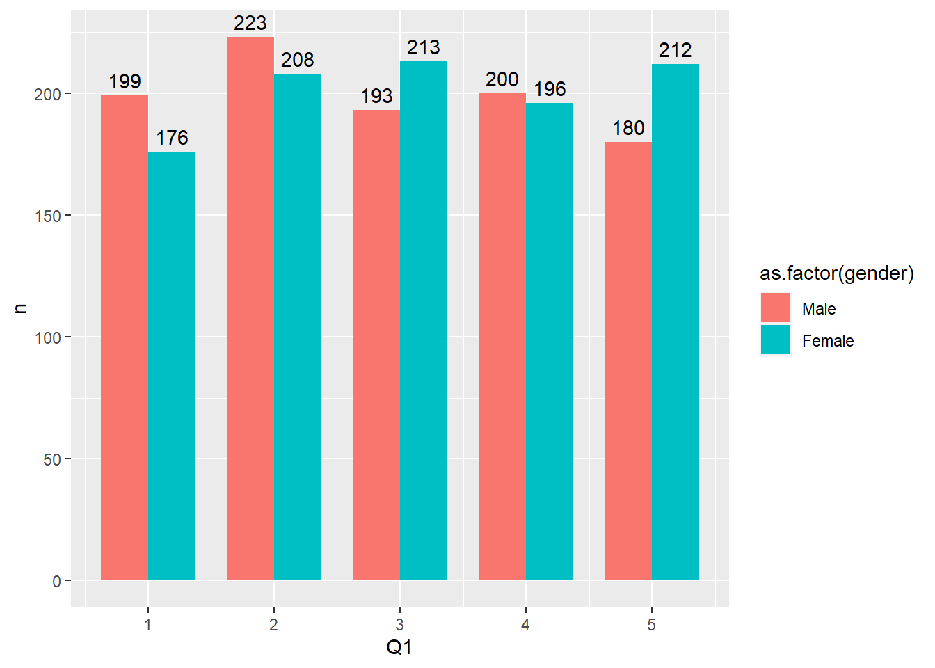
Figure 6.8: Satisfaction with Store by Gender
6.2.2 Formatting Charts Using Themes
Now that we have a chart with specified values, we can make it nicer by adding a theme that specifies how the text should look on the x-axis along with labels for x and y axis as follows:
# By specifying as.factor for Q1 we can see the labels on X-axis
# Using theme, we can specify positioning of elements of X-axis
# adding ylim to specify values for y axis for better visibility of chart values
ggplot(newdata, mapping=aes(x=as.factor(Q1),y=n,fill=as.factor(gender)))+
  geom_bar(stat="identity",position=position_dodge(0.75),width=0.75)+
  geom_text(aes(label=n),vjust=-0.5,position=position_dodge(0.75))+
  ggtitle("Satisfaction with Store by Gender Formatted Using Theme")+
  xlab("Satisfaction with Store")+
  ylab("Count")+
  theme(axis.text.x = element_text(hjust=1,angle=45, size=12), axis.title = element_text(size=13, face="bold"), title=element_text(size=13, face="bold"))+
  ylim(0,250)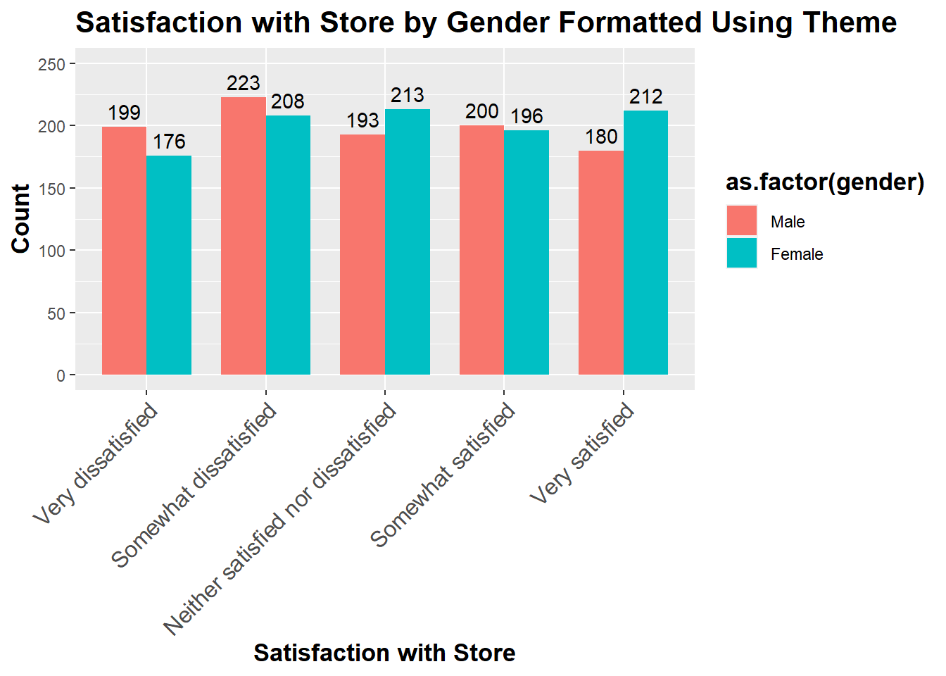
Figure 6.9: Satisfaction with Store by Gender Formatted Using Theme
As seen in the chart above, theme can be used to make many other modifications to look of the labels and legend.
6.2.3 Visualizing Data by Group
There is another nice chart feature in ggplot that makes it possible to see differences by group. By adding the option of facet, it is possible to see the value of Q1 separately by group as follows with slight modification to the syntax used before:
# using facet_wrap to wrap the data by gender
ggplot(newdata, mapping=aes(x=as.factor(Q1),y=n,fill=as.factor(gender)))+
  geom_bar(stat="identity",position=position_dodge(0.75),width=0.75)+
  geom_text(aes(label=n),vjust=-0.5,position=position_dodge(0.75))+
  ggtitle("Satisfaction with Store by Gender Using Facet Wrap")+
  xlab("Satisfaction with Store")+
  ylab("Count")+
  theme(axis.text.x = element_text(hjust=1,angle=45))+
  ylim(0,250)+
  facet_wrap(~as.factor(gender))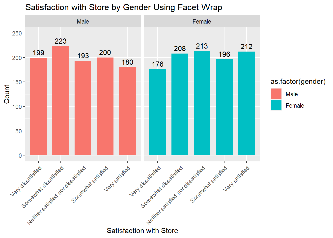
Figure 6.10: Satisfaction with Store by Gender using Facet Wrap
By viewing the chart in this manner, it is clear that a greater proportion of females is in general, more satisfied while the chart for males shows them leaning more toward dissatisfaction.
6.3 Other Types of Plots
Although ggplot package offers many types of plots, we will just discuss a few here that might be handy to a beginner. For the sake of simplicity, we will ignore formatting options so the reader may focus on the ggplot layers.
6.3.1 Creating a Density Plot
Another way of looking at the difference in satisfaction with store between males and females is using a density plot as follows:
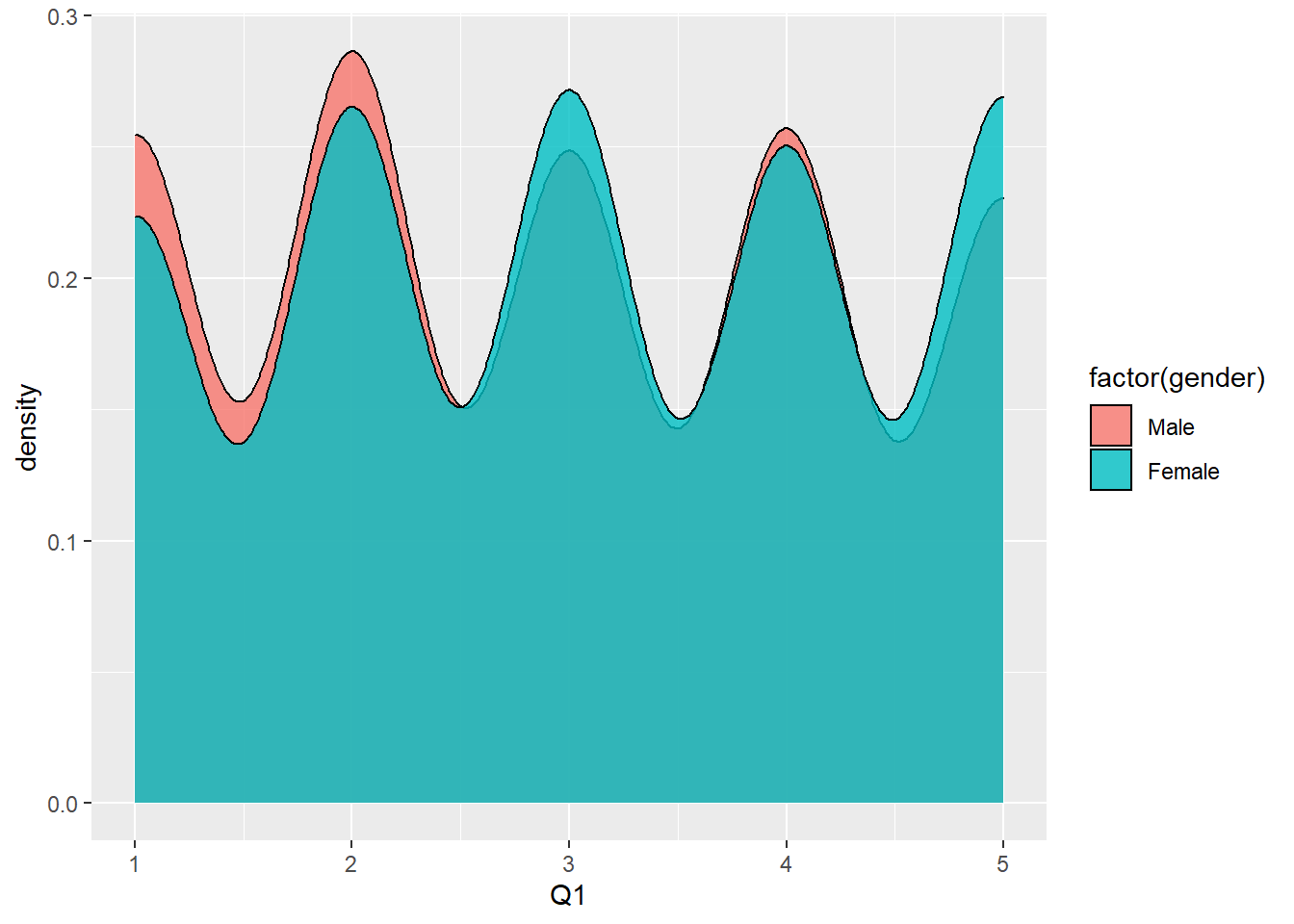
Figure 6.11: Density Chart of Satisfaction with Store by Gender
The argument alpha defines the level of transparency in colors between the two groups.
6.3.2 Creating a Jitter Plot
Some of these plots are better in case of continuous variables. For example, geom_point provides a scatterplot; however it does not work as well for categorical variables or variables that are integers as Q1 happens to be. In this case, we may use geom_jitter which scatters the points so they are not overlapping as follows:
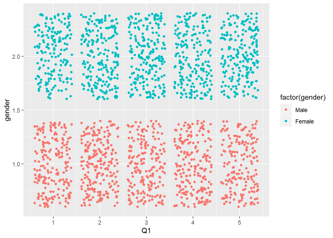
Figure 6.12: Jitter Plot of Satisfaction with Store by Gender
6.3.3 Creating a Box Plot and Violin Plot
Since the satisfaction scores are evenly distributed across, there is not much difference to be seen in the jitter plot. However, it offers another way of presenting the data when differences are more obvious.
Since variable Q5 measures whether customers are likely to recommend to others, we can use a boxplot to look at the data by gender as follows:
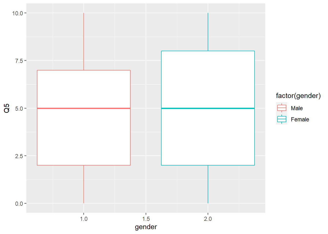
Figure 6.13: Box Plot of Likelihood to Recommend by Gender
The boxplot shows some differences between males and females. However, it does not show the density of values at each point. A violin plot which is similar to a box plot also shows the density as follows:
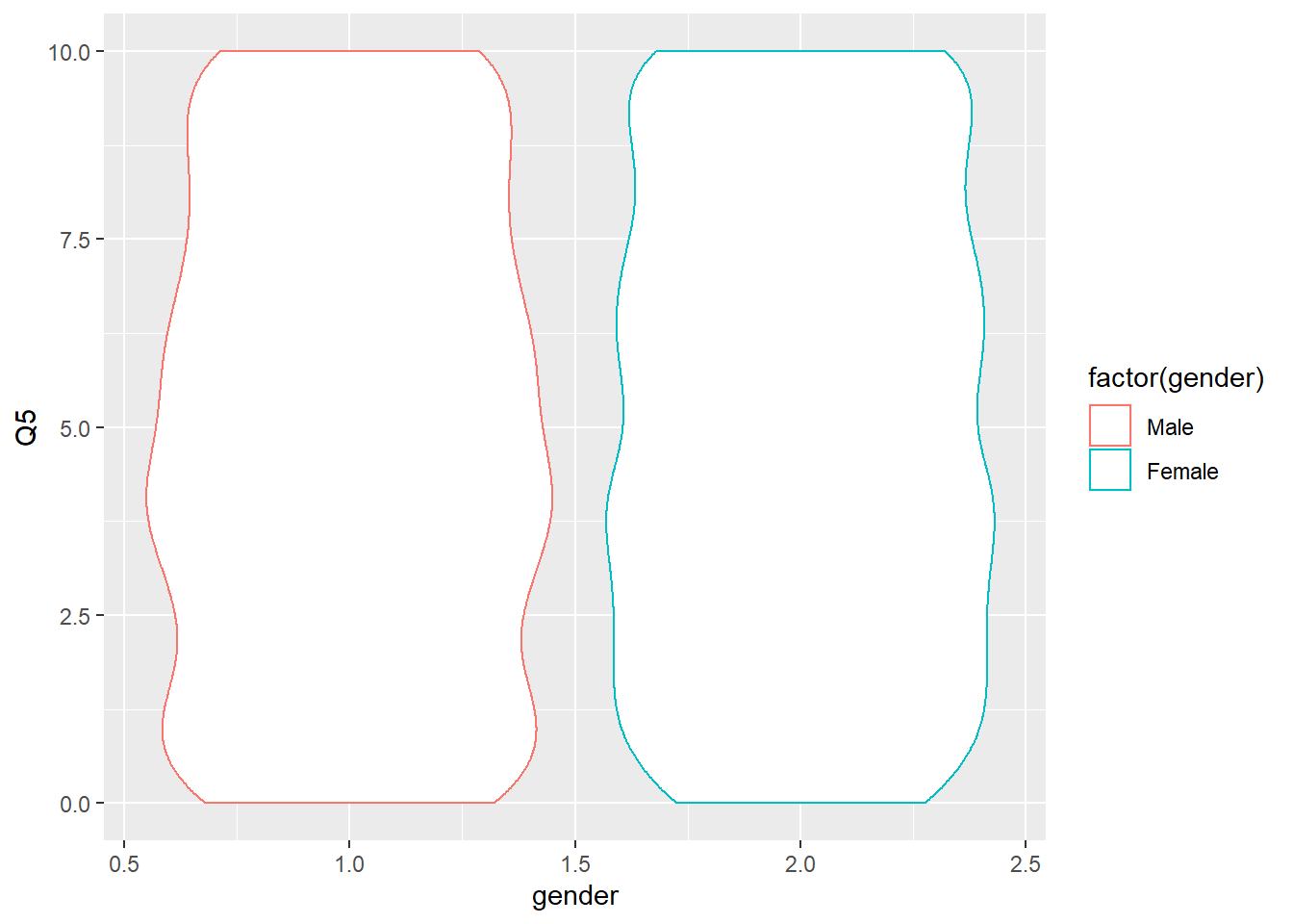
Figure 6.14: Violin Plot of Likelihood to Recommend by Gender
The violin plot shows a slightly greater protruberance in values less than 5 for males, indicating they are less likely to recommend.
In summary, in Chapter 6 you have seen a variety of ways in which data may be visualized and presented, along with how to make it aesthetically pleasing as well.
Demin, Gregory. 2020. Expss: Tables, Labels and Some Useful Functions from Spreadsheets and ’Spss’ Statistics. https://CRAN.R-project.org/package=expss.
Hainke, Michael. 2018. Getting Started Using Survey Data for Analysis. https://www.hainke.ca/.
R Core Team. 2020. R: A Language and Environment for Statistical Computing. Vienna, Austria: R Foundation for Statistical Computing. https://www.R-project.org/.
Wickham, Hadley. 2015. R Packages: Organize, Test, Document, and Share Your Code. 1st ed. Sebastopol, California: O’ Reilly Media Inc. http://r-pkgs.had.co.nz/intro.html.
Wickham, Hadley, Romain François, Lionel Henry, and Kirill Müller. 2020. Dplyr: A Grammar of Data Manipulation. https://CRAN.R-project.org/package=dplyr.
Wickham, Hadley, and Garrett Grolemund. 2017. R for Data Science. 1st ed. Sebastopol, California: O’ Reilly Media Inc. https://r4ds.had.co.nz/.
Xie, Yihui. 2020. Bookdown: Authoring Books and Technical Documents with R Markdown. https://CRAN.R-project.org/package=bookdown.