Chapter 4 Using R’s Basic Functions

This chapter will walk the reader through R-Studio’s user interface’s basic functions and packages. The previous chapters focused on what R is, how to install R-Studio and R, and a general overview of its user interface. In this chapter, you will learn how to use R and some basic commands for defining variables and creating data sets. Before you can start reading, manipulating, and analyzing data, it is important to understand how R interprets data. Creating, saving, and then retrieving the dataset created will provide a preliminary understanding of how R handles data.

4.1 Creating a Project and Setting Working Directory

Before launching into creating a dataset, it is important to understand how R handles data from a filing and directory perspective. Before creating a dataset, R starts with creation of a ‘new project.’ A project name is a name given to a folder that will hold everything that is associated with a specific project such as data, history of commands used, objects (In R a variable and/or data are stored as “objects”) or variables that are created.

Along with creating a new project name, it is important to understand the concept of working directory as R will look for variables and objects or any other files that are being called in the working directory. A simple way to check on what the current working directory is, is to type the command getwd() into the command console. If it is not the intended directory you want to use, the simplest way to change it is by using “viewer” pane and clicking on the tab that says ‘more.’ Ensuring that your working directory is where you want your files and objects created to be stored is important, especially to a beginner.

For the purpose of this book, you may now create a new project by opening R-Studio, clicking on file, and then ‘new project.’ As shown in Figure 4.1 the window that opens asks if you would like to open the project in an existing directory, a new one, or simply version control. Existing directory is the directory that is currently the working directory. You may either choose an existing directory or a new one. However, if you choose a new one, you need to make sure that it is selected as the working directory as shown earlier. You may name your project as ‘Learning R.’

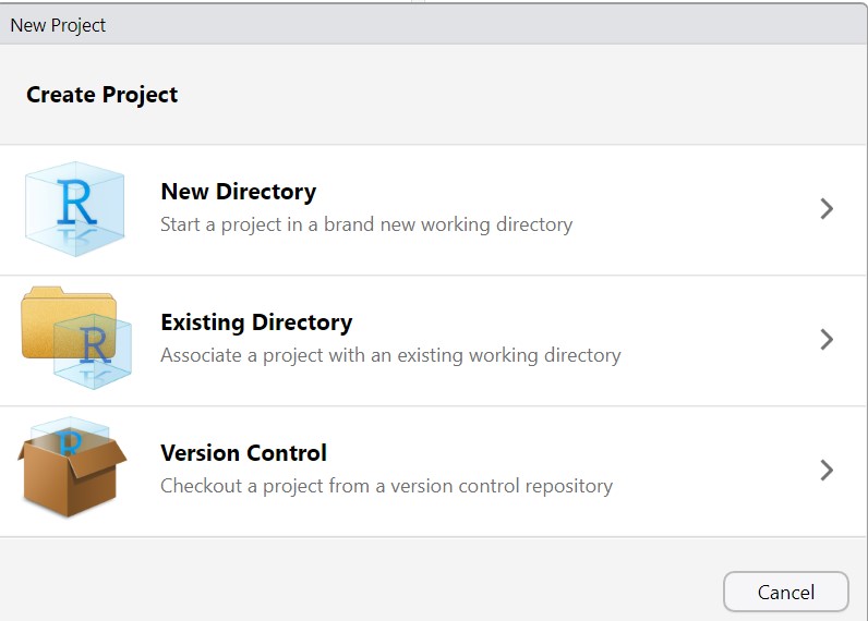
Figure 4.1: Interface for Creating a Project in R

Once the project is created, you will see a .proj file under the files section in the viewer pane as shown in Figure 4.2. As the figure shows, a new proj called ‘Learning R.rproj’ has been created in the directory /home/R/books/Learning R. Any work done will now be stored in this directory (by setting it as the working directory) and in this project as long as it is saved when you exit.

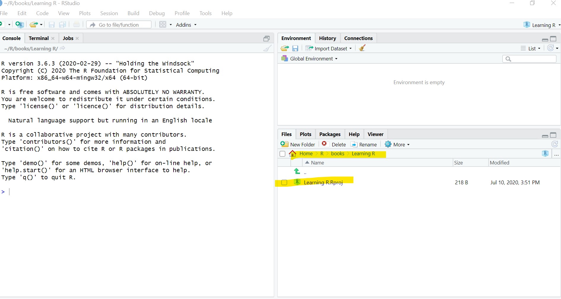
Figure 4.2: Directory with New Project

4.2 Creating a Simple Data Set in R

Now that the new project is created, the next step is to create a simple data frame to save as a dataset and then retrieve it in R, as most analyses entail some variation of such tasks. R treats variables a little differently if you are used to using Excel or other statistical packages such as SPSS. A little understanding of how it treats variables and the terminology that is used in R is necessary here.

In R, variables are assigned values as follows using the <- sign. Typing x into the R console brings up the value of 2 as shown below.

x<-2
x

## [1] 2

While x was assigned a single value in the above example, it is also possible to create a vector (a sequence of different values assigned to a variable) as follows. This is useful when we are creating a variable with multiple values based on multiple observations.

x<-c(2,4,6,8,10)
x

## [1]  2  4  6  8 10

As seen above, using the command above, x is now a vector (a sequence of values). The top right part of your R-Studio console will show x as a data object, a numeric variable with 5 different values.

While x is a numeric variable, we can also assign character values such as names as follows:

y<-c('a','b','c','d','e')
y

## [1] "a" "b" "c" "d" "e"

Again looking at your global environment in the top right pane of your console, you will find that two variables have been created, a numeric variable x and a character variable called y as shown in Figure 4.3 below.

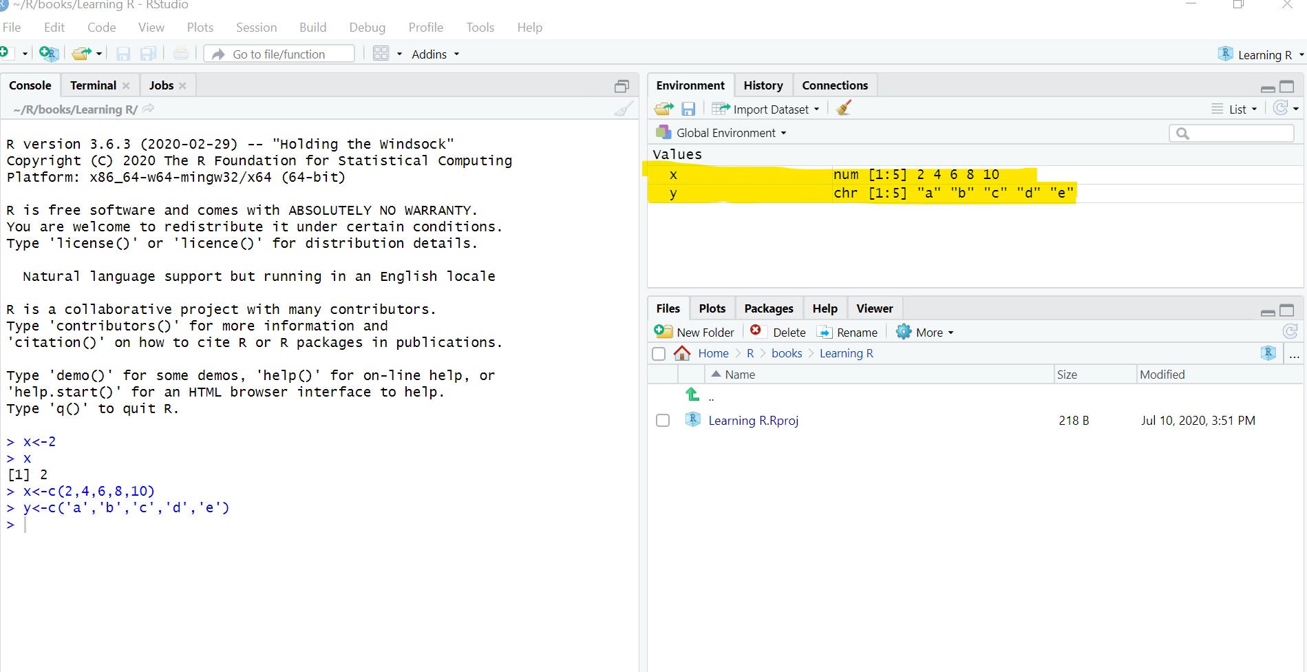
Figure 4.3: Global Environment with Variables

Another way to check the nature of the variable is to simply type in class(x) in the command line and it shows that x is a numeric variable.

Now that there are two variables with five values each, it is possible to combine them as a data frame (which is data stored as rows and columns) and save it as a file. A data frame when created is stored as an object as will be seen in the global environment in the top right pane of the console. A simple way to refer to the data frame is ‘df’, although it may be given any name the user chooses for convenience and clarity.

Data frame is a base function within R. When the words data.frame are typed into the console, R-Studio automatically shows what the function does and how it is to be used. As described, the function data.frame allows for “creation of collection of tightly coupled collection of variables often used as the fundamental data structure by most of R modeling software.” Thus, a data frame with two variables y and x is created as follows. As shown below, typing in ‘df’ which is the name assigned here to the data frame shows that we now have a dataset with two columns and five observations.

df<-data.frame(y,x)
df

##   y  x
## 1 a  2
## 2 b  4
## 3 c  6
## 4 d  8
## 5 e 10

Although this data frame is available as a dataframe object within R in our newly created project, there are times when we would like to save it as a dataset for retrieval later. It is possible to save the data in different formats. In this particular example, we will save it as a csv file as follows:

write.csv(df,file="learnRdata.csv")

The above command saves the dataframe object ‘df’ as a .csv file in the working directory. Since we have the directory of the learningR project as the working directory, the data file just saved should be available in the directory. The data from this file maybe read into the project as a new object as an example on how to retrieve or read in a data set using the read built in function in R as follows:

df2<-read.csv(file="learnRdata.csv")
df2

##   X y  x
## 1 1 a  2
## 2 2 b  4
## 3 3 c  6
## 4 4 d  8
## 5 5 e 10

Not assigning the read data to an object means that it will not be available for manipulation. Since we did not specify that there are no row names, R automatically added a new column for row names called X1. To avoid this, we can use the argument as follows:

write.csv(df,file = "learnRdata.csv",row.names = FALSE)
df2<-read.csv(file= "learnRdata.csv")
df2

##   y  x
## 1 a  2
## 2 b  4
## 3 c  6
## 4 d  8
## 5 e 10

Thus, we have now created variables with values, transformed them into a dataset, and read the dataset back as an object. A look at the global environment displays all the objects created so far which is useful when trying to understand what variables and objects (which could be variables or data frames or other types of objects) are available for use within the environment. In the next section, we will take a look at some other built in functions of R.

4.3 Using R’s Built-in Functions

R, as already seen, has a number of built in functions. Some functions are basic mathematical ones such as addition, subtraction, multiplication, and division. For example, if we create a new variable with a value of 10, we could modify the new variable through simple mathematical transformations as follows:

newvar<-10
##adding 2
newvar+2

## [1] 12

##subtracting 2
newvar-2

## [1] 8

## multiplying by 2
newvar*2

## [1] 20

##dividing by 2
newvar/2

## [1] 5

Some of the statistical functions available are measures of central tendency and dispersion such as mean, median, and standard deviation. For numeric variables, it is possible to compute all of the important measures with one single command using the summary function as follows:

summary(x)

##    Min. 1st Qu.  Median    Mean 3rd Qu.    Max. 
##       2       4       6       6       8      10

Please note, that to use any of this derived output later, it needs to be assigned to a variable or an object for later retrieval. For example, ‘newvar’ on which we performed different operations, will only have the value of 10, its original assigned value, unless it is assigned to a new variable, perhaps called ‘newvar2’ when performing computations.

Thus, R has many built in base functions that are useful for exploratory data analysis. For a quick list of the type of built-in functions, see the highlighted table below. There are others such as lm for in base function which is of interest to someone interested in analysis using models. However, this chapter only covers some basic functions for quick exploration of the data.

Quick Guide to Built-in Statistical Functions in R

Mean(x): compute mean of variable x
Median(x): compute median of variable x
Sd(x): compute standard deviation of numbers in vector x
Scale(x): Compute z-scores of numbers in vector x
Quantile(x): Compute the quartiles or percentiles of numbers in vector x
Var(x,y=null): computes variance of variable x or covariance or correlation for x and y.
Cov(x,y)
Cor(x,y)

In the next chapter, we will use some of the functions learned about in this chapter to both manipulate and analyze a dataset.