Chapter 8 Random Number Generation
Sheldon: I’ll create an algorithm that will generate a pseudorandom schedule. Do you know why it will not be a “true” random schedule?
Amy: Because the generation of true random numbers remains an unsolved problem in computer science?
- Big Bang Theory, Season 12, Episode 1
Many of the methods in computational statistics require the ability to generate random variables from known probability distributions.
Random numbers have been used for thousands of years in decision-making, divination, and games. Ancient civilizations cast lots, rolled dice, and drew straws; Babylonians held lotteries, while Greeks and Romans used dice for leisure and governance.
With the rise of gambling in the 17th and 18th centuries, randomness gained prominence in games of chance, coinciding with the development of probability theory by mathematicians like Pascal and Fermat.

But gambling aside, randomness has many uses in science, statistics, cryptography and more.
The use of random numbers in statistics has expanded beyond random sampling or random assignment of treatments to experimental units. More common uses now are in simulation studies of stochastic processes, analytically intractable mathematical expressions, or a population by resampling from a given sample from that population.
In this section, we explore how to generate random numbers using computers.
8.1 How do computers do it?
Using dice, coins, or similar media as a random device has its limitations.
Thanks to human ingenuity—and computers—we have more powerful tools and methods at our disposal.
The 20th century saw the shift from mechanical methods to electronic ones, with early computers generating random numbers for scientific applications such as the Manhattan Project.
Random numbers play a crucial role in computing, simulations, cryptography, and statistical sampling. However, not all random numbers are created in the same way.
Let’s consider first the two principal methods used to generate random numbers: true random numbers and pseudorandom numbers.
True Random Numbers
Definition 8.1 True Random Numbers are based on a physical process, and harvests the source of randomness from some physical phenomenon that is expected to be random.
Such a phenomenon takes place outside of the computer. It is measured and adjusted for possible biases due to the measurement process.
Examples include the following.
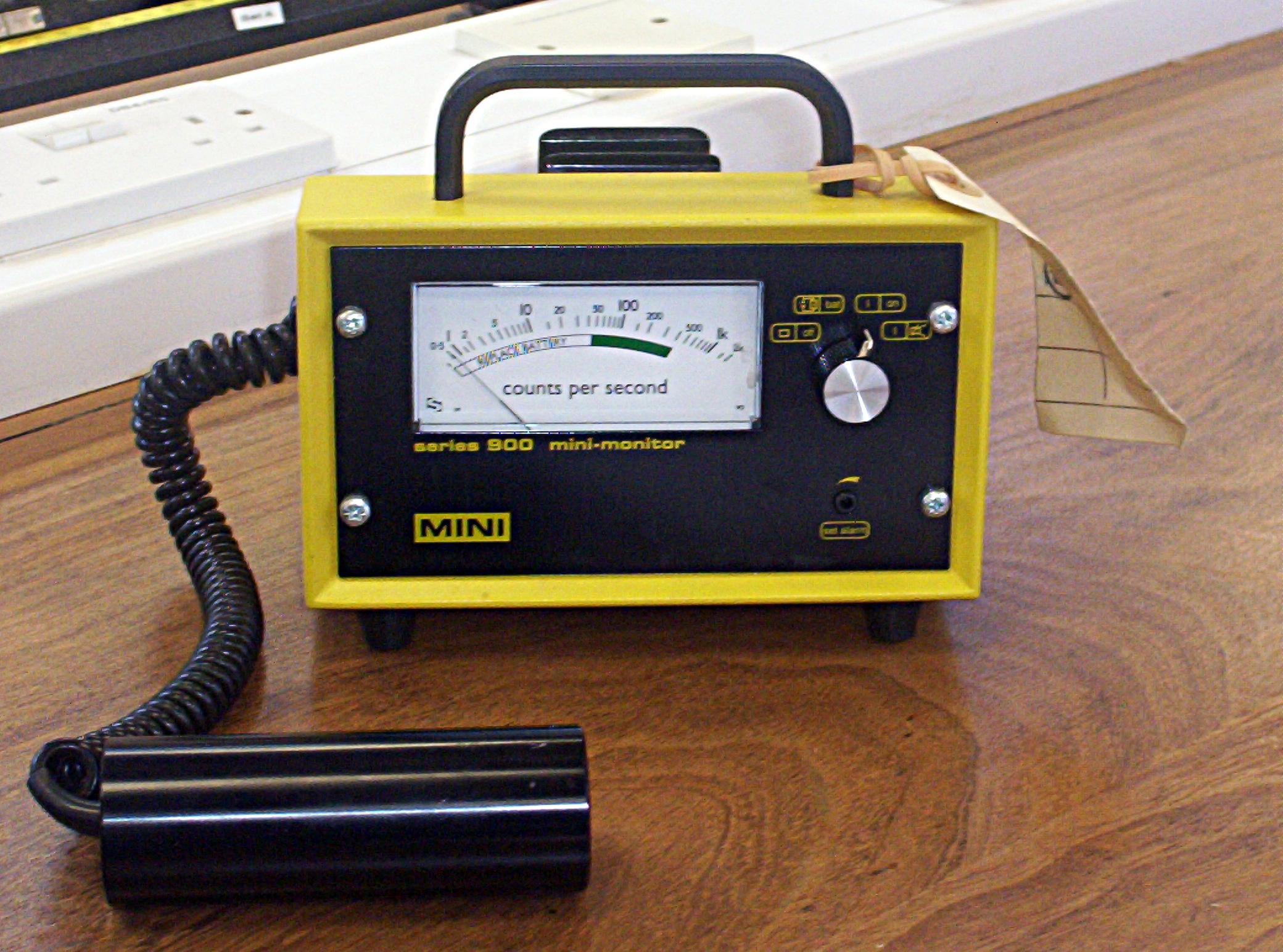
Radiation decay: The decay of unstable atomic nuclei is fundamentally unpredictable. This is detected by a Geiger counter (an electronic instrument used for detecting and measuring ionising radiation) attached to a computer.
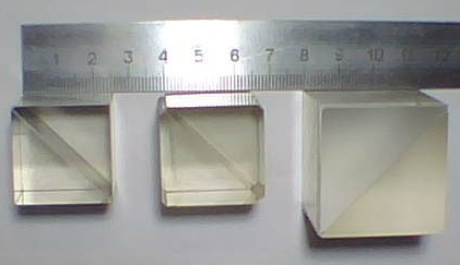
Photon Measurements: Photons travelling through a semi-transparent mirror (or a beam splitter). The mutually exclusive events (reflection/transmission) are detected and associated to ‘0’ or ‘1’ bit values respectively.
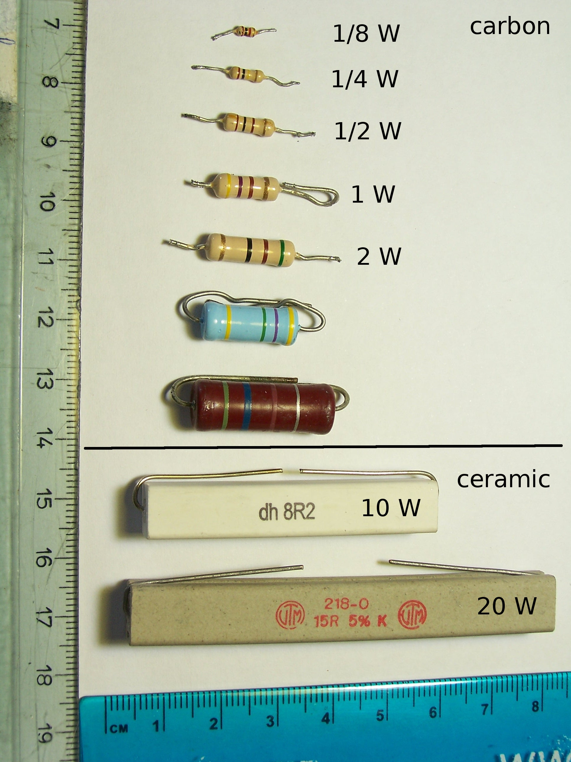
Thermal noise: Random fluctuations in electrical circuits due to temperature variations. Thermal noise from a resistor are amplified to provide a random voltage source.
Thus, random numbers generated based on such randomness are said to be “true” random numbers.
Pseudorandom Numbers
As an alternative to “true” random numbers, the second method of generating random numbers involves computational algorithms that can produce apparently random results.
Why apparently random? Because the end results obtained are in fact completely determined by an initial value also known as the seed value or key. Therefore, if you knew the key value and how the algorithm works, you could reproduce these seemingly random results.
Definition 8.2 Pseudorandom numbers (PRNs) are generated by deterministic algorithms that produce sequences of numbers that appear random but are fully determined by an initial value, known as a seed.
Because of the deterministic nature of PRNGs, they are useful when you need to replay a sequence of random events. This helps a great deal in code testing and simulations, for example.
On the other hand, TRNGs are not periodic and work better in security sensitive roles such as encryption.
A period is the number of iterations a PRNG goes through before it starts repeating itself. Thus, all other things being equal, a PRNG with a longer period would take more computer resources to predict and crack.
In R, the default algorithm for generating random numbers has a period of \(2^{19937}−1\) This means that \(2^{19937}−1≈4.3154×10^{6001}\) random numbers are generated by the algorithm before the algorithm repeats itself.
To summarize:
| Feature | True Random Numbers | Pseudorandom Numbers |
|---|---|---|
| Source | Physical Process | Algorithmic Computation |
| Reproducability | No | Yes (with seed) |
| Speed | Slower | Faster |
| Security | High | Lower |
| Usage | Cryptography, security | Simulations, Modelling |
In most statistical and computational contexts, pseudorandom numbers are sufficient, but for security-sensitive applications, true randomness is preferred.
8.2 General techniques for Generating Random Variables
In this section, we will demonstrate some methods of generating pseudorandom numbers in computers.
Linear Congruential Generator
Uniform Random Number Generator
Inverse Transform Method
Box-Muller Algorithm
Other Transformation Methods
R has built in functions that generate numbers from a specified distribution. However, the following algorithms will be very useful for implementation in other situations, such as a C program.
The Linear Congruential Generator
Preliminaries: The modulo operator
The modulo operator finds the remainder when one number is divided by another. Mathematically, for integers \(a\) and \(m\):
\[ a \mod m \quad =\quad \text{remainder of } \frac{a}{m} \] Properties of the Modulo Operator
Modulo Bounds
The result of \(a \mod m\) is always between \(0\) and \(m-1\)
\[ 0 \leq (a \mod m) < m \]
In the following demonstration, we will see that the value of \(a \mod 3\) will just be from \(0\) to \(2\).
## [1] 1 2 0 1 2 0 1 2 0 1 2Periodicity
Any integer shifted by multiples of \(m\) has the same remainder.
\[ (a + km) \mod m \quad =\quad a \mod m \]
## [1] 1
## [1] 1
A more general demonstration, let \(a =7\) and \(m = 3\):
## [1] 1Now, showing for different values of \(k\), we expect that \((7 + k \times 3 ) \text{ mod } 3 = 1\)
## [1] 1 1 1 1 1
Now, using this concept, we create an algorithm that generates a series of pseudorandom numbers.
Definition 8.3 (Linear Congruential Generator) Given an initial seed \(X_0\) and integer parameters \(a\) as the multiplier, \(b\) as the increment, and \(m\) as the modulus, the generator is defined by the linear relation:
\[ X_n =(aX_{n-1}+b) \quad \text{mod} \quad m \]
The output is a sequence \(\{X_n\}\) containing pseudorandom numbers.
Each of these members have to satisfy the following conditions:
\(m > 0\) (the modulus is positive)
\(0 < a < m\) (the multiplier \(a\) is positive but less than the modulus \(m\)).
\(0 \leq b < m\) (the increment \(b\) is nonnegative but less than the modulus), and
\(0 \leq X_0 < m\) (the seed \(X_0\) is nonnegative but less than the modulus).
Let’s create an R function that takes the initial values as arguments and returns an array of random numbers of a given length.
lcg <- function(seed, a, b, m, n) {
    # Pre-allocate vector for efficiency
    x <- numeric(n+1)
    x[1] <- seed
    for (i in 2:(n+1)) {
        x[i] <- (a * x[i-1] + b) %% m
    }
    return(x)
}
# Example: Parameters from Numerical Recipes (a common choice)
seed <- 12345
a <- 1664525
b <- 1013904223
m <- 2^32
n <- 10
lcg(seed, a, b, m, n)## [1] 12345 87628868 71072467 2332836374 2726892157 3908547000 483019191 2129828778 2355140353
## [10] 2560230508 3364893915Alternatively, you can have a recursive function instead of a for loop
lcg_r <- function(seed, a, c, m, n) {
    # Base case: stop recursion when n = 0
    if (n == 0) {
        return(seed)
    }else{

        # Compute next random number
        next_val <- (a * seed + c) %% m

        # Recursively call with updated seed
        return(c(seed, lcg_r(next_val, a, c, m, n - 1)))
    }
}

lcg_r(seed, a, b, m, n)
## [1] 12345 87628868 71072467 2332836374 2726892157 3908547000 483019191 2129828778 2355140353
## [10] 2560230508 3364893915Key considerations:
The modulus
mis often a very large prime number or power of 2 (e.g. \(2^{31}-1\) or \(2^{32}\)).The multiplier
aaffects the change in output for a unit increase in seed number.The increment
bdetermines the distance of numbers between each other in a single run of the algorithm.Poor choices of \(a,b,m\) can lead to poor randomness, producing patterns in the output vector.
\((a X_0 + b) \mod m\) should not be equal to \(X_0\), otherwise, you will have the following:
## [1] 2 2 2 2 2 2 2 2 2 2 2 2 2 2 2 2 2 2 2 2 2 2 2 2 2 2The sequence below has low periodicity, with the pattern repeating at \(X_{17}\)
## [1] 7 6 1 8 11 10 5 12 15 14 9 0 3 2 13 4 7 6 1 8 11 10 5 12 15 14We want a very high value for the modulo \(m\) so that the sequence needs to be very long before the elements repeat.
##  [1]   1 110 616  20 556 980 196 740  36 300  76 660 316 820 756 780 396 540 236 100 276 460 516 620
## [25] 956 580 596 340 436 900 476
How do we make this more random?
As mentioned, this is just a pseudorandom number: every time we run the function, the output is the same.
What if we include a factor that the user (theoretically) cannot control, and may change every time the random generator is executed?
Even though pseudorandom number generators typically doesn’t gather any data from sources of naturally occurring randomness, such gathering of keys may be made random when needed. For example, getting the computer time or some number from a true random number generator as a seed number.
For this, we use the time of the computer.
In R, Sys.time() is a function that shows the current date time of the computer.
## [1] "2025-12-18 14:31:34 PST"If we apply the as.integer function to a POSIXct object, it gets the number of seconds since the Unix epoch (1970-01-01 00:00:00 UTC)
## [1] 0Since we are in the Philippines, this gets the number of seconds since 1970-01-01 08:00:00 PST
## [1] 0How do we make a random number out of this?
Every second that you run as.integer(Sys.time()), you will get a different number:
as.integer(Sys.time())
profvis::pause(1)
as.integer(Sys.time())
profvis::pause(1)
as.integer(Sys.time())
## [1] 1766039494
## NULL
## [1] 1766039495
## NULL
## [1] 1766039496We will make the computer system time as our default seed number.
lcg_2 <- function(n = 1,  seed = as.integer(Sys.time())) {
    a <- 1664525
    b <- 1013904223
    m <- 2^32

    numbers <- numeric(n)
    x <- seed
    for (i in 1:n) {
        x <- (a * x + b) %% m
        numbers[i] <- x
    }
    return(numbers)
}
Now, every second that you run the following, you will get a different result:
## [1] 554680455 4263543866 40814161 3707521916 1517170859If you want a fixed value every time, you just set the value of the seed number:
## [1] 3980087773 3919915416 4164722711 2710257290 115743841You can also gather the seed number from a true random number generator. The following random number generator is from random.org, where the randomness comes from atmospheric noise.
The following function obtains a random integer from this site.
getRandom <- function(min = 1, max = 1000, base = 10) {
  url <- paste0(
    "https://www.random.org/integers/?num=1",
    "&min=", min,
    "&max=", max,
    "&col=1",
    "&base=", base,
    "&format=plain",
    "&rnd=new"
  )

  # Use httr for request
  response <- httr::GET(url)

  # Extract the content as text and convert to numeric
  number <- as.numeric(httr::content(response, as = "text", encoding = "UTF-8"))
  return(number)
}
You need internet to call this function.
## [1] 834Integrating with the LCG:
## [1] 2184065298 186031433 727778836 2965125731 3907804262## [1] 1138743598 349392565 741544080 1907370671 1585043522NOTE: Even if the seed number is truly random, the sequence generated by the LCG is still not truly random since the elements are not independent from each other
Uniform Random Numbers
Most methods for generating random variables start with random numbers that are uniformly distributed on an interval. We denote this by \(U\).
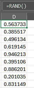
In Excel, the function =RAND() returns a random number greater than or equal to 0 and less than 1, evenly distributed.
Now, we modify the Linear Congruential Generator such that it will only output values from 0 to 1.
Recall that the \(m-1\) is the maximum possible value generated by LCG, from the properties of the modulo operator, before it circles back to 0. We normalize the generated vector \(\{X_n\}\) to \([0,1]\) by dividing the elements by \(m-1\).
lcg_unif <- function(n = 1,
                     seed = as.integer(Sys.time())) {

    a <- 1664525123
    b <- 1013904223
    m <- 2^32-1

    numbers <- numeric(n)
    x <- seed
    for (i in 1:n) {
        x <- (a * x + b) %% m
        numbers[i] <- x
    }
    return(numbers/(m-1)) # normalize to [0,1]
}## [1] 0.8253023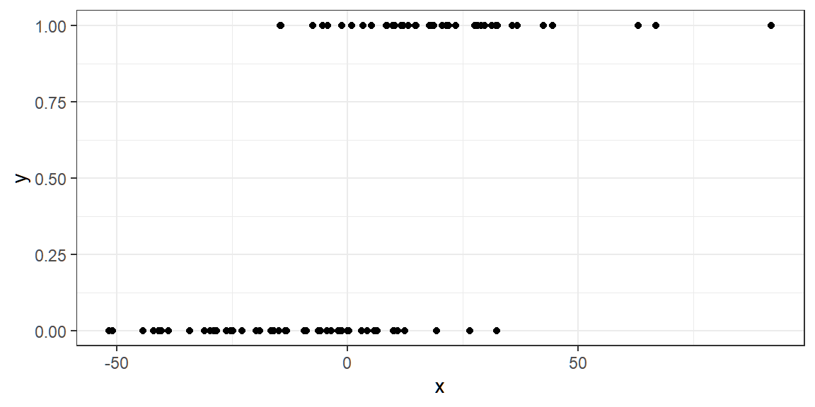
If \(U\sim Uniform(0,1)\), then any uniformly distributed randomly variable over an interval \(a\) and \(b\) may be generated by a simple transformation:
\[ X=(b-a)\cdot U+a \sim Uniform(a,b) \]
For example, we want to generate a (continuous) random number from 10 to 20:
Inverse Transform Method
Recall Probability Integral Transform in your Stat 122 class.
Theorem 8.1 (Probability Integral Transform) If \(X\) is a continuous random variable with cdf \(F_X\), then the random variable \(F^{-1}(U)\), where \(U\sim Uniform(0,1)\), has distribution \(F_X\).
We can use this concept to generate a random variable from a specified distribution, assuming that we can derive the inverse of its cumulative distribution function.
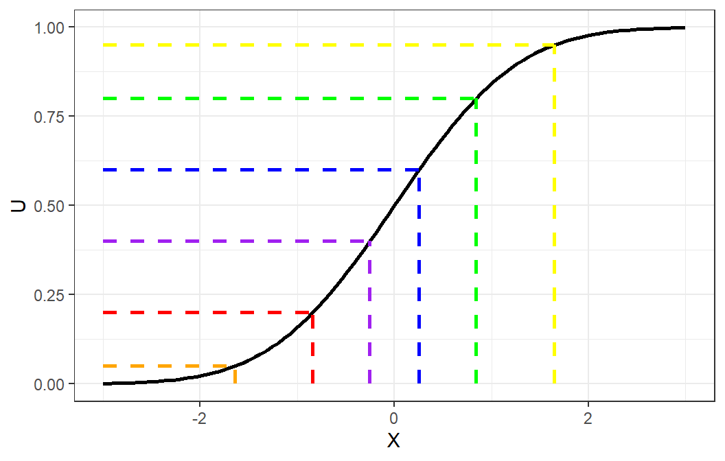
Inverse Transform Method (Continuous Case)
Derive the expression for the inverse distribution function \(F^{-1}(U)\).
Generate standard uniform number \(U\).
Obtain desired \(X\) from \(X=F^{-1}(U)\)

Inverse Transform Method (Discrete Case)
Define a probability mass function for \(x_i\), \(i=1,\dots,k\). Note that \(k\) could grow infinitely.
Generate a uniform random number \(U\).
If \(U\leq p_0\), set \(X=x_0\)
else if \(U \leq p_0 + p_1\), set \(X = x_1\)
else if \(U \leq p_0 + p_1 + p_2\), set \(X=x_2\)
\(\vdots\)
else if \(U \leq p_0 + p_1 + \cdots + p_k\), set \(X=x_k\)
Example: Discrete Distribution
We would like to simulate a discrete random variable \(Y\) that has probability mass function given by
\[ P(Y=0) = 0.3 \\ P(Y=1) = 0.2 \\ P(Y=2) = 0.5 \]
The CDF is
\[ F(y)=\begin{cases} 0 & y<0 \\ 0.3 & 0 \leq y < 1 \\ 0.5 & 1 \leq y < 2 \\ 1.0 & 2 \leq y \end{cases} \]
We generate the random variable \(Y\) according to the following scheme:
\[ Y=\begin{cases} 0 & U\leq 0.3 \\ 1 & 0.3 < U \leq 0.5 \\ 2 & 0.5 < U \leq 1 \end{cases} \]
In R, the
case_whenfunction from thedplyrlibrary is convenient for transforming values from a vector.
LIMITATION: The inverse transform method is only useful if the inverse of the CDF of a random variable has a closed form.
Can we use this method to generate data from the Normal distribution?
Box-Muller Algorithm
The following algorithm helps us with generating numbers from a Normal Distribution, given that we can generate Uniform Random Numbers.
Definition 8.4 (Box-Muller Algorithm) Generate \(U_1\) and \(U_2\), two independent \(Uniform(0,1)\) random variables, and set
\[ R = \sqrt{-2 \log{U_1}} \quad \text{and} \quad \theta =2\pi U_2 \]
Then
\[ X = R \cos(\theta) \quad \text{and}\quad Y = R \sin (\theta) \]
are independent \(Normal(0,1)\) random variables.
Although we have no quick transformation for generating a single \(N(0,1)\), this is a method for generating two \(N(0,1)\) random variables.
Unfortunately, solutions such as the Box-Muller algorithm are not plentiful. Moreover, they take advantage of the specific structure of certain distributions and are, thus, less applicable as general strategies.
Other Transformation Methods
Many types of transformations other than the probability inverse transformation can be applied to simulate random variables. Some examples are:
If \(Z\sim N(0,1)\), then \(V=Z\sim \chi^2(1)\).
If \(U\sim\chi^2(m)\) and \(V\sim \chi^2(n)\) are independent, then \(F=\frac{U/m}{V/n}\sim F(m,n)\)
If \(Z\sim N(0,1)\) and \(V\sim \chi^2(n)\) are independent, then \(T=\frac{Z}{\sqrt{V/n}}\) has the student’s T distribution with \(n\) degrees of freedom.
If \(X_1,...,X_\alpha \overset{iid}{\sim} Exp(\lambda)\), then \(Y=\sum_{i=1}^\alpha X_i\sim Gamma(\alpha,\lambda)\)
If \(U\sim Gamma(r,\lambda)\) and \(V \sim Gamma(s,\lambda)\) are independent, then \(X = \frac{U}{U+V}\) has the \(Beta(r,s)\) distribution.
If \(U,V\sim Unif(0,1)\) are independent, then
\[ X= \left\lfloor 1+\frac{\log (V)}{\log ( 1-(1-\theta)^U )} \right\rfloor \]
is the \(Logarithmic(\theta)\) distribution, where \(\lfloor x \rfloor\) is the integer part of \(x\)
(Optional) Acceptance Rejection Method
The problem with the Inverse Transform method is that the CDF must have a closed form and the inverse must be derivable.
This cannot be achieved in some cases.
Suppose that \(X\) and \(Y\) are random variables with density with density pmf \(f\) and \(g\) respectively, and there exists \(c\) such that
\[ \frac{f(t)}{g(t)}\leq c \]
for all \(t\) such that \(f(t)>0\). Then the acceptance-rejection method (or rejection method) can be applied to generate the random variable \(X\). It is required that there is already a method to generate \(Y\).
Procedure: Acceptance-Rejection Method (Continuous Case)
Choose a density \(g(y)\) that is easy to sample from, preferrably a known and common distribution.
Find a constant \(c\) such that \[ \frac{f(t)}{g(t)}\leq c \] is satisfied.
Generate a random number \(Y\) from the density \(g(y)\).
Generate a uniform random number \(U\).
If
\[ U\leq \frac{f(Y)}{cg(Y)} \]
then accept \(X = Y\). Else, go to step 3.
8.3 Random Number Generation in R
R provides convenient functions for simulating and analyzing random variables from many probability distributions.
Before discussing those methods, however, it is also useful to summarize some of the probability functions available in R. The probability mass function (pmf) or density (pdf), cumulative distribution function (cdf), quantile function, and random generator of many commonly used probability distributions are available.
R provides four types of functions that follow a consistent naming scheme:
dfoo: density or probability mass (pdf/pmf)pfoo: cumulative distribution function (cdf)qfoo: quantile functionrfoo: random number generation
Where foo is the name of the distribution.
For example, the normal distribution functions are dnorm(), pnorm(), qnorm(), and rnorm().
Before the end of this chapter, a table summarizes common distributions and their corresponding functions.
sample will also be introduced, which is used to obtain sample elements from a vector.
Random Generation
Functions beginning with r generate random samples. This is useful for simulation studies.
# Generate 1000 random values from a normal distribution
x <- rnorm(1000, mean = 0, sd = 1)


# Plot histogram
ggplot(data.frame(x), aes(x = x))+
    geom_histogram(aes(y = after_stat(density)), bins = 15)+
    theme_minimal()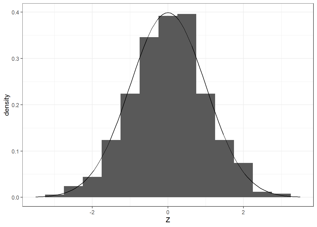
Other examples:
runif(1000, min = 0, max = 1)generates uniform random numbers.rbinom(1000, size = 10, prob = 0.3)generates binomial outcomes.
Probability Density and Mass Functions
Functions beginning with d evaluate the probability density (continuous) or mass (discrete) of a distribution at given values.
## [1] 0.3989423## [1] 0.2668279These functions are useful for overlaying theoretical curves on histograms.
ggplot(data.frame(x), aes(x = x))+
    geom_histogram(aes(y = after_stat(density)), bins = 15) +
    stat_function(fun = dnorm, args = list(mean = 0, sd = 1),
                  color = "blue") +
    theme_minimal() +
    xlim(-3,3)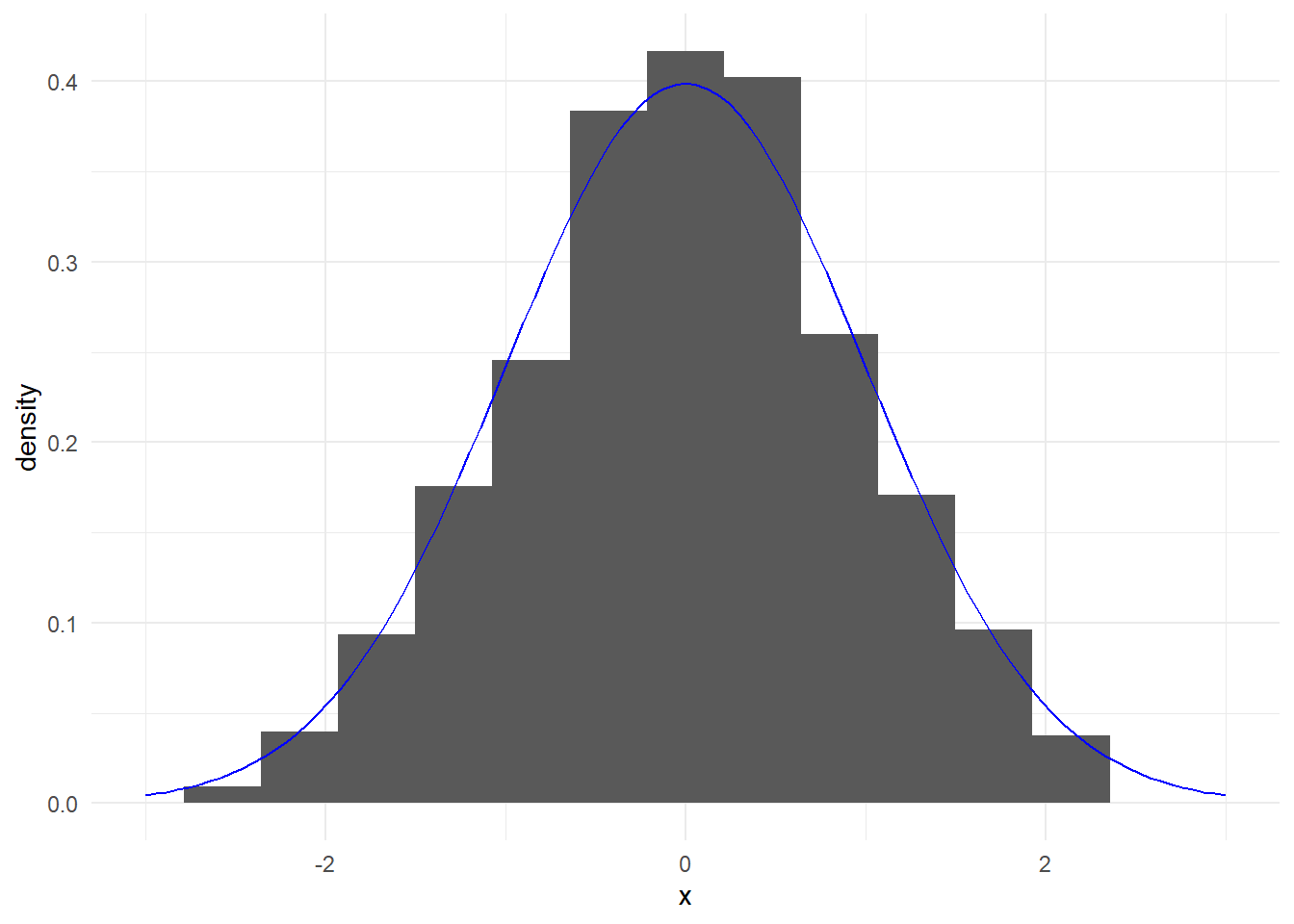
Cumulative Distribution Functions
Functions beginning with p return the probability that a random variable is less than or equal to a given value.
## [1] 0.9750021## [1] 0.6496107We can use this function to plot the cdf.
# Visualize normal CDF
x <- seq(-3, 3, 0.1)

ggplot(data.frame(x), aes(x)) +
    stat_function(fun = pnorm, args = list(mean = 0, sd = 1),
              color = "red", size = 1) +
    labs(title = "CDF of Standard Normal", y = "P(X ≤ x)", x = "x")
ggplot(data.frame(x), aes(x)) +
    stat_function(fun = pbinom,
                  args = list(size = 10, prob = 0.3),
                  color = "red", size = 1) +
    labs(title = "CDF of Binomial(n=10, p = 0.3)", y
         = "P(X ≤ x)", x = "x")+
    xlim(0,10)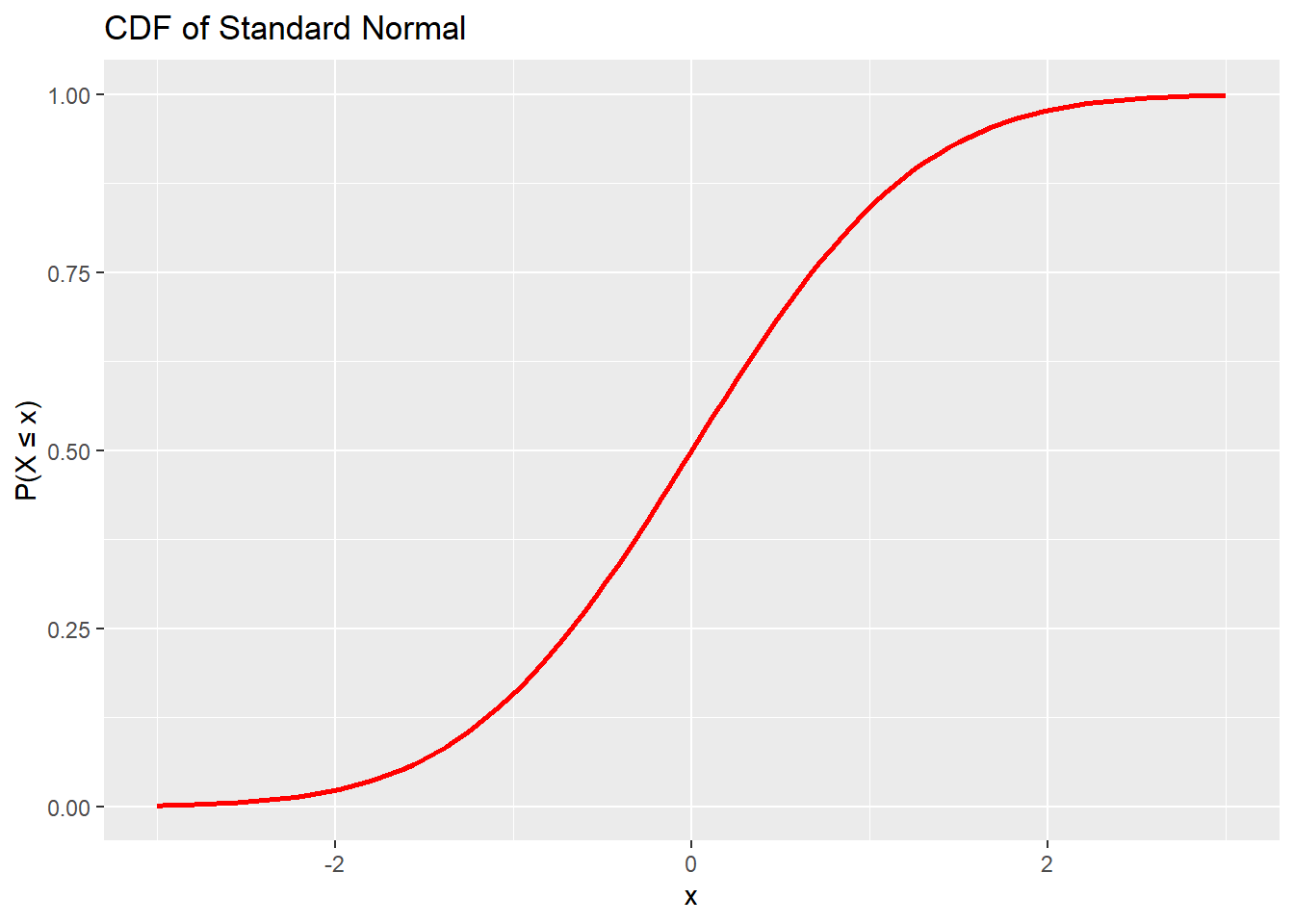
Quantile Functions
Functions beginning with q give the cutoff value corresponding to a given probability.
## [1] 1.644854## [1] 0.5Quantile functions are useful for simulation, threshold determination, and constructing confidence intervals (recall PQM).
Summary of Functions
The table below provides a partial list of probability distributions and their parameters. For a complete list, see the R documentation .
| Distribution | cdf | generator | parameters |
|---|---|---|---|
| \(Beta(\alpha, \beta)\) | pbeta |
rbeta |
shape1, shape2 |
| \(Binomial(n,p)\) | pbinom |
rbinom |
size, prob |
| \(\chi^2(\text{df})\) | pchisq |
rchisq |
df |
| \(Exponential(\lambda)\) | pexp |
rexp |
rate |
| \(F(\text{df}_1,\text{df}_2)\) | pf |
rf |
df1, df2 |
| \(Gamma(\alpha,\lambda)\) | pgamma |
rgamma |
shape, rate |
| \(Geometric(p)\) | pgeom |
rgeom |
prob |
| \(\textit{NB}(r,p)\) | pnbinom |
rnbinom |
size, prob |
| \(Normal(\mu,\sigma)\) | pnorm |
rnorm |
mean, sd |
| \(Poisson(\lambda)\) | ppois |
rpois |
lambda |
| \(T(\text{df})\) | pt |
rt |
df |
| \(\textit{Uniform}(min,max)\) | punif |
runif |
min, max |
In addition to the parameters shown, many functions also accept optional arguments such as log, lower.tail, or log.p, and some support an additional ncp (noncentrality) parameter.
sample
This function is used to generate a random element from a vector.
Generate a random name from a vector of names.
## [1] "Anna"Generate a sample of size 10 from sequence of integers from 1 to 100, without replacement:
## [1] 42 22 41 83 7 80 34 76 12 28Generate a sample of size 10 from sequence of integers from 1 to 15, with replacement:
sample(1:15, size = 10, replace = T)
sample(1:15, size = 10, replace = T)
sample(1:15, size = 10, replace = T)
## [1] 5 6 1 6 9 6 6 2 9 8 ## [1] 9 10 9 6 5 9 9 2 6 12 ## [1] 10 6 6 12 5 10 8 4 10 1Bernoulli Experiment, where
TRUEis success,FALSEis failure, with probability of success \(p=0.7\).## [1] FALSE10 independent and identical Bernoulli trials.
replace=Tensures that each element in the sample are IID.## [1] TRUE TRUE FALSE TRUE TRUE TRUE TRUE TRUE TRUE TRUE
Exercises
The Cauchy Distribution has the following CDF
\[ F(x)=\frac{1}{\pi}\tan^{-1}\left(\frac{x-\theta}{\gamma}\right) + \frac{1}{2} \]
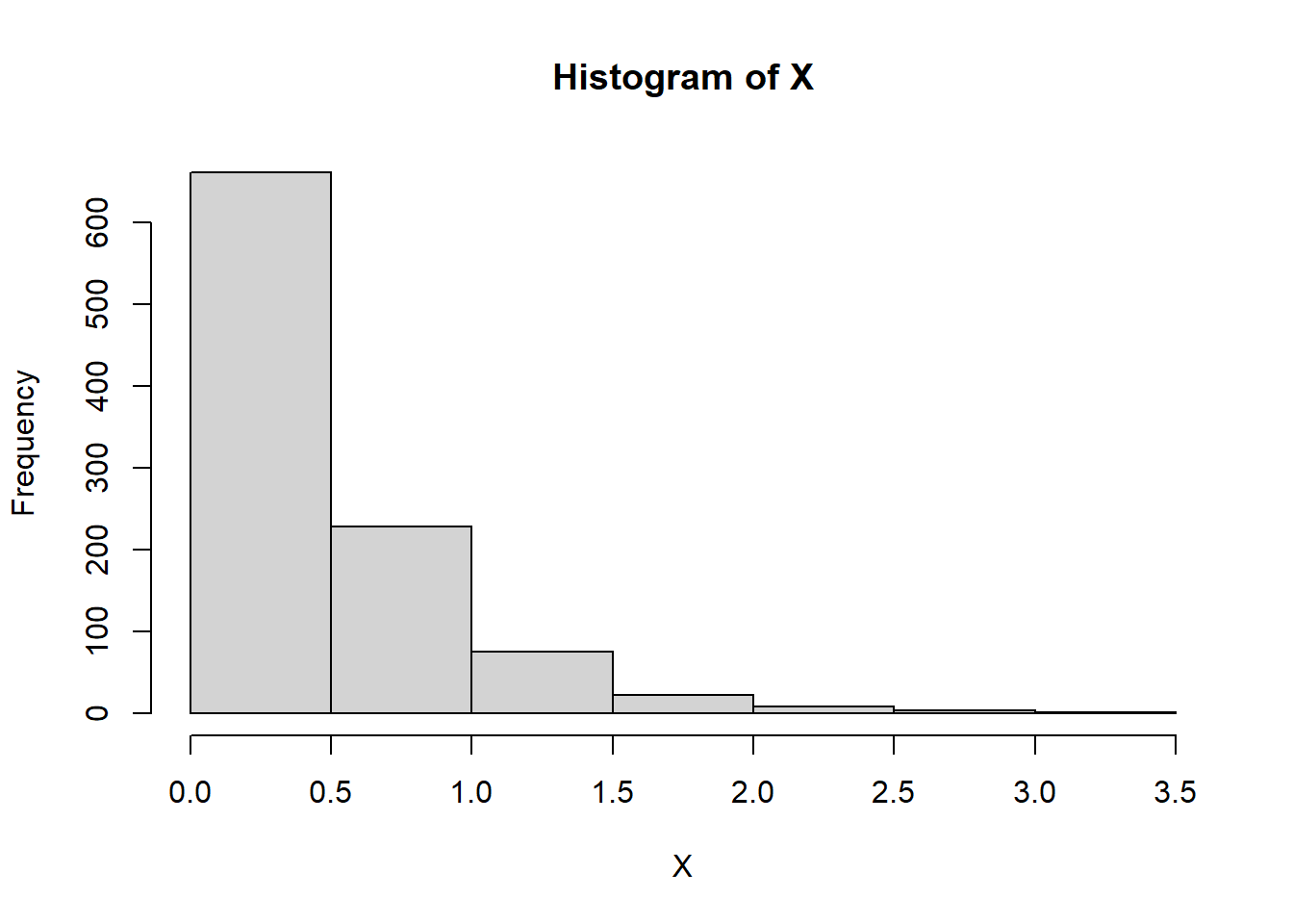
Derive its inverse \(F^{-1}(u)\), and obtain a sample from \(Cauchy(\theta=0,\gamma=1)\). Use
lcg_unif(n=1000)for generating numbers from \(Unif(0,1)\).Obtaining random observations from a dataset
Explore the dataset
mtcarsIt has 32 rows and 11 columns.
Obtain a random sample of size 5 by sampling from the vector
1:32, and using dataframe indexing, and thesamplefunction. Use142as your seed number.Generating Random Numbers from a Linear Model
Suppose we want to simulate from the following linear model
\[ y_i = \beta_0 +\beta_1x_i+\varepsilon_i \]
where \(\varepsilon_i \overset{iid}{\sim} N(\mu = 0, \sigma^2 = 2^2)\).
The variable \(x\) might represent an important predictor of the outcome \(y\)
Assume that \(x\) is a constant in the integer range \([1,100]\), \(\beta_0 = 0.5\) and \(\beta_1=2\).
Generate a value of \(y\) for each level of \(x\). Use
142as your seed number.Store values of
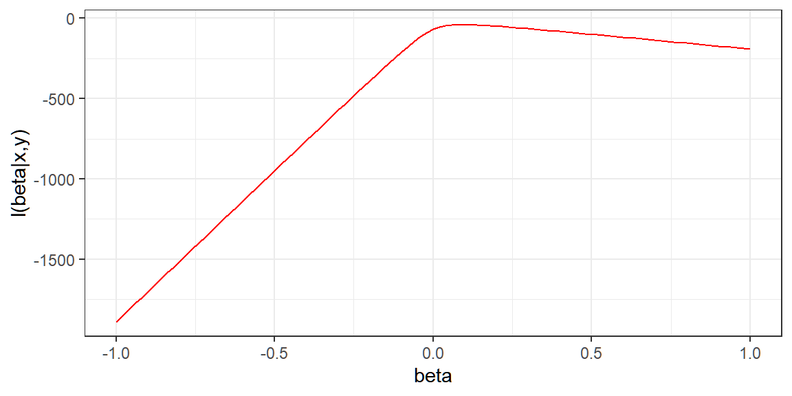
yandxon adata.frameobject.Estimate values of \(\beta_0\) and \(\beta_1\) using OLS.
Plot the values of \(x\) and \(y\)
(Preparation for Monte Carlo)
Recall from Stat 136, \(\hat{\beta_1}\) is BLUE and UMVUE of \(\beta_1\). If \(\varepsilon \sim N(0,2^2)\), assuming known variance, what is the distribution of \(\hat{\beta_1}\)?
Perform steps i. to iii. in Exercise 3 \(100\) times to generate \(100\) values of \(\hat{\beta_1}\).
Plot a histogram of the generated values, and overlay the theoretical pdf of \(\hat{\beta_1}\) assuming known variance.
References
The outline of this chapter is adapted from handouts of Asst. Prof. Xavier Bilon. Contents related to statistical theory are from the following resources:
Casella, G., & Berger, R. L. (2002). Statistical inference. Brooks/Cole.
Gentle, J. E. (2003). Random number generation and Monte Carlo methods (2nd ed.). Springer. Arobelidze, A. (2020, October 26).
Random number generator: How do computers generate random numbers?. https://www.freecodecamp.org/news/random-number-generator/
Rizzo, M. L. (2007). Statistical Computing with R. In Chapman and Hall/CRC eBooks. https://doi.org/10.1201/9781420010718