Chapter 10 Monte Carlo Experiments

Definition 10.1 Monte Carlo Simulations are a class of computational algorithms that rely on repeated random sampling to estimate numerical results.

They are widely used in various fields, including statistics, physics, finance, and machine learning, to approximate complex mathematical problems that may not have closed-form solutions.

A Monte Carlo Simulation or Experiment is also useful in evaluating the impact of certain conditions (non-normality, model misspecification etc.) on statistical methods (about estimation, prediction etc.) based on some score (MSE, Bias, MAPE etc.)

Monte Carlo Simulation is just a computer EXPERIMENT

For our class, the following is the proposed outline for creating a Monte Carlo Experiment

Set up scenarios (design space)

Define your objective (what question to answer).

Choose key factors and reasonable levels.

Specify the data-generating process for each scenario.

Select performance metrics (score function)

Pick measures tied to the objective (bias, MSE, SE, power, coverage, accuracy, etc.).

Decide how results will be summarized (averages, MC-SE, plots).

Include a diagnostic check (e.g., type I error when null is true).

Identify comparison methods

Establish a baseline (control), usually the most common methodology used

Add alternative(s) for evaluation.

Fix parameters/settings in advance.

Summarize

Monte Carlo methods can be applied to estimate parameters of the sampling distribution of a statistic, mean squared error (MSE), percentiles, or other quantities of interest.

It also can be designed to assess the coverage probability for conﬁdence intervals, to ﬁnd an empirical Type I error rate of a test procedure, to estimate the power of a test, and generally, to compare the performance of different procedures for a given problem.

This chapter will help you design Monte Carlo experiments that are grounded on statistical inference.

Methods for evaluating point estimators, interval estimators, and hypothesis tests are from Casella & Berger (2002). Examples are derived from handouts of Bilon (2021) and Supranes (nd).

In a Monte Carlo experiment, we can assess the performance of an estimator by repeatedly simulating data from a known population, allowing us to approximate its sampling distribution, standard error, bias, and mean squared error.

Random variates from the sampling distribution of an estimator \(\hat{\theta}\) can be generated by repeatedly drawing independent random samples \(\textbf{x}_m\) and computing \(\hat{\theta}_m\) = \(\hat{\theta}(x_{1(m)}, . . . , x_{n(m)})\) for each sample.

10.1 Sampling Distribution of a Statistic

One type of problem that arises frequently in statistical applications is the need to evaluate the cdf of the sampling distribution of a statistic, when the density function of the statistic is unknown or intractable.

Recall from Section 9.2 and Theorem 9.1, the empirical cdf.

Definition 10.2 A Monte Carlo estimate of the sampling distribution of a statistic is

\[ P(\hat{\theta} \leq t)\approx F_M(t)=\frac{1}{M}\sum_{m=1}^MI(\hat{\theta}_m\leq t) \]

Example: Central Limit Theorem

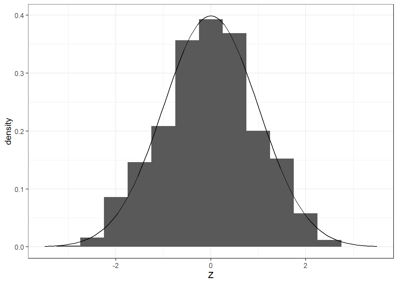
As an example, we visualize distribution of the statistic

\[ \frac{\bar{X}_n-\mu}{\sigma/\sqrt{n}} \] By the Central limit theorem, we know that this approaches the standard normal distribution, for a random sample \(X_1,X_2,...,X_n\) from a population with mean \(\mu\) and finite variance \(\sigma^2\).

Suppose the population has a distribution \(Poisson(\lambda = 6)\). The mean and variance are both \(\lambda = 6\).

Let’s obtain a random sample of size \(n=30\) repeatedly and examine the distribution of the statistic \(\frac{\bar{X}-\mu}{\sigma/\sqrt{n}}\).

Here, we use the replicate function. This is a faster way than using loops when conditions are the same each iteration and the goal is to generate a vector.

M <- 1000
n <- 30
Z <- replicate(M, 
               {X <- rpois(n, lambda = 6)
               (mean(X) - 6)/sqrt(6/n)
               })

It looks standard normal, doesn’t it?

Suppose we obtained the following sample from the population:

set.seed(142)
samp <- rpois(n, lambda = 6)

Computing \(\frac{\bar{X}-\mu}{\sigma/\sqrt{n}}\) using this sample, wehave:

z <- (mean(samp) - 6)/sqrt(6/n)
z

## [1] 1.565248

By the central limit theorem, \(P(Z \leq 1.57)\approx \Phi(1.57)=0.9412\)

pnorm(z)

## [1] 0.9412376

But using Monte-Carlo Simulation, we count how many samples will have a Z-statistic that are less than the observed Z-statistic

sum(Z <= z)/M

## [1] 0.938

Close enough?

This Monte Carlo approach is more useful if the probability distribution of a statistic has no closed form, or has no theorem that support convergence in distribution. Try to explore the distribution of other statistics, like the statistics used in non-parametric inference (e.g. Wilcoxon Signed-Rank Statistic, Wilcoxon Rank-Sum / Mann–Whitney U Statistic, Kruskal–Wallis H Statistic, Spearman’s Rank Correlation Coefficient, Kendall’s Tau, etc…)

10.2 Monte Carlo Methods for Evaluating Estimators

Inferential statistics draws conclusions about a population based on an estimator that can be computed using a sample. Recall that a parameter can have different estimators, and a difficulty that arises when we are faced with the task of choosing between estimators.

Bias of a point estimator

Recall that the bias of an estimator \(\hat{\theta}\) of a parameter \(\theta\) is the difference between the expected value of \(\hat{\theta}\) and \(\theta\); that is, \(Bias_\theta(\hat{\theta})=\mathbb{E}(\hat{\theta})-\theta\). It is difficult to obtain the bias if you don’t know the expectation of an estimator.

By law of large numbers, if you have \(M\) replicates of \(\hat{\theta}\), then \(\frac{1}{M}\sum_{m=1}^M \hat{\theta}_m\rightarrow\mathbb{E}(\hat{\theta})\)

Definition 10.3 A Monte Carlo estimate for the bias of an estimator \(\hat{\theta}\) in estimating \(\theta\) is

\[ \widehat{Bias}_\theta(\hat{\theta})=\frac{1}{M}\sum_{m=1}^M \hat{\theta}_m-\theta \]

Example

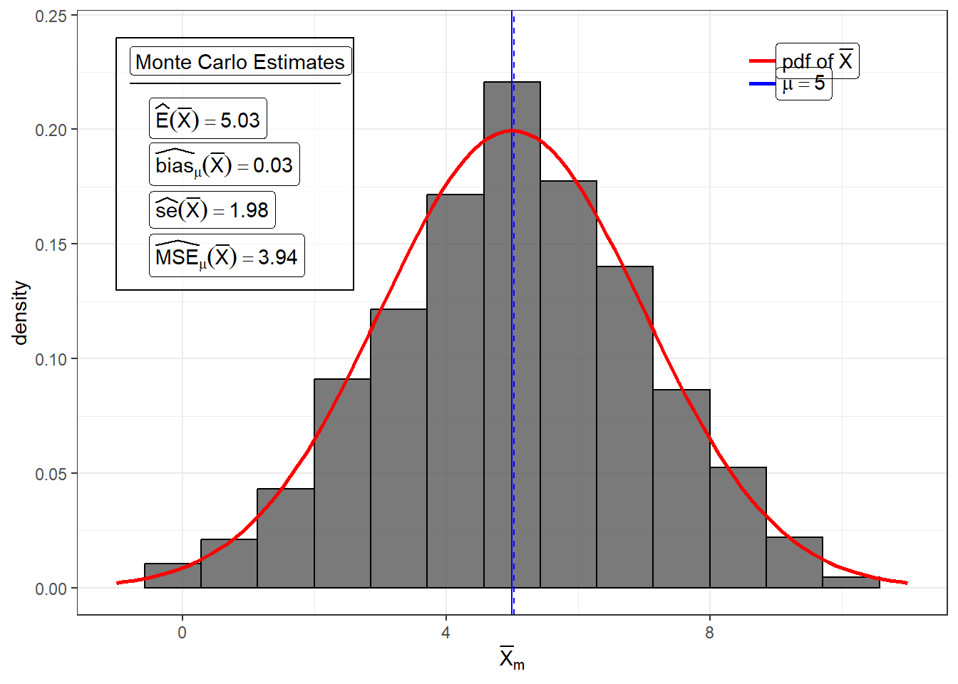
For example, we know that the the sample mean \(\bar{X}\) is unbiased for \(\mu\). Suppose \(X_1,...,X_{25}\sim N(\mu = 5, \sigma^2 = 100)\), then \(Bias_\mu(\bar{X})=0\).

set.seed(142)
M <- 1000
xbar <- replicate(M, mean(rnorm(25, mean = 5, sd = 10)))
bias_xbar <- mean(xbar) - 5
bias_xbar

## [1] 0.03515856

Standard Error of a Statistic

Suppose \(\hat{\theta}\) is an estimator of \(\theta\). We can obtain a Monte Carlo estimate of its standard error by obtaining \(M\) samples of this statistic.

Definition 10.4 A Monte Carlo estimate for the variance of a statistic \(\hat{\theta}\)

\[ \widehat{Var}(\hat{\theta}) =\frac{1}{M}\sum_{m=1}^M(\hat{\theta}_m-\bar{\hat{\theta}})^2 \] and a Monte Carlo estimate for the standard error of a statistic \(\hat{\theta}\)

\[ \widehat{se}(\hat{\theta}) = \sqrt{\frac{1}{M}\sum_{m=1}^M(\hat{\theta}_m-\bar{\hat{\theta}})^2} \] where \(\bar{\hat{\theta}}\) is the sample mean of the \(\hat{\theta}_m\)s

Note: You may use \(M\) or \(M-1\) in the denominator.

In other words, you may use the formula for the sample variance and sample standard deviation. Difference will be negligible anyway for large \(M\)*

Example

For example, we know that the standard error of the sample mean \(\bar{X}\) is \(\sigma/\sqrt{n}\). Suppose \(X_1,...,X_{25}\sim N(\mu = 5, \sigma^2 = 100)\), then \(se(\bar{X})=2\).

set.seed(142)
M <- 1000
xbar <- replicate(M, mean(rnorm(25, mean = 5, sd = 10)))

var_xbar <- mean((xbar-mean(xbar))^2)
var_xbar

## [1] 3.940161

se_xbar <- sqrt(var_xbar)
se_xbar

## [1] 1.984984

MSE of a point estimator

Recall that the mean square error (MSE) of an estimator \(\hat{\theta}\) of a parameter \(\theta\) is defined by \(\mathbb{E}(\hat{\theta}-\theta)^2\)

Monte Carlo methods can be applied to estimate the MSE of an estimator.

Definition 10.5 A Monte Carlo estimate of the \(MSE\) of an estimator \(\hat{\theta}\) of parameter \(\theta\) is

\[ \widehat{MSE}_\theta(\hat{\theta}) = \frac{1}{M}\sum_{m=1}^M(\hat{\theta}_m-\theta)^2 \]

where \(\hat{\theta}_m\) is the estimate obtained using the \(m^{th}\) random sample \(\{x_1,...,x_n\}_m\)

Example

Following the same example for \(\bar{X}\)

set.seed(142)
M <- 1000
xbar <- replicate(M, mean(rnorm(25, mean = 5, sd = 10)))
mse_xbar <- mean((xbar-5)^2)
mse_xbar

## [1] 3.941397

Decomposition of MSE

Note: the MSE can be decomposed as the sum of the variance and square of the bias

\[ \mathbb{E}_\theta(\hat{\theta}-\theta)^2 = Var(\hat{\theta}) + Bias_\theta(\hat{\theta})^2 \]

The empirical results of the simulation proves this.
var_xbar + bias_xbar^2
## [1] 3.941397
mse_xbar
## [1] 3.941397
This only works if you use the same seed number and simulation settings for the computation of the Monte Carlo estimates of Variance, Bias, and MSE.

Exercise

Suppose we want to investigate the distribution of sample standard deviation (SD) of a size \(n = 200\) random sample from a \(Normal(2, 1)\).
- Using Monte Carlo Simulation with \(M = 1000\), show the relative frequency histogram of the distribution of sample SD.
- Based on the simulation, what is the estimated mean and variance of the distribution of sample SD?
Create functions bias_mc,

Example: Mean of Poisson

Suppose our population is best modelled by a Poisson distribution (commonly used for count data). The Poisson distribution is completely described by a single parameter: rate, \(\lambda = \mu\).

The question here is

“Is the sample mean still unbiased and does it have lower variance than other estimators, say sample median?”

In this example, we will compare the bias and variance of the two estimators, sample mean and sample median in estimating the population mean for populations distributed as Poisson at different sample sizes and at different values of the parameter \(\lambda\).

Obtain a sample of size \(n\) from the Poisson population.
From the generated sample, compute the sample mean and sample median.
Do this for \(M\) times to obtain \(M\) sample means and \(M\) sample medians.
From these \(M\) values, compute the mean and variance of the sample mean and sample median so we can assess their bias and variance respectively.

See full results and source code of this example in UVLe.

10.3 Monte Carlo Methods for Evaluating Tests

Suppose that we wish to test a hypothesis concerning a parameter \(\theta\) that lies in a parameter space \(\Theta\). The hypotheses of interest are \[ H_0:\theta \in \Theta_0 \quad \text{vs} \quad H_1:\theta\in\Theta_1 \]

where \(\Theta_0\) and \(\Theta_1\) partition the parameter space \(\Theta\).

(Recall) Two types of error can occur in statistical hypothesis testing:

Type I error: Reject Ho when it is in fact true
Type II error: Do not reject Ho when it is in fact false.

The signiﬁcance level of a test, denoted by \(\alpha\), is an upper bound on the probability of Type I error. The probability of rejecting the null hypothesis depends on the true value of \(θ\), whether it is in \(\Theta_0\) or \(\Theta_1\) (hopefully higher if \(\theta\in\Theta_1\)).

Let \(\pi(\theta)\) denote the probability of rejecting \(H_0\). Then

\[ \alpha = \sup_{\theta\in\Theta_0} \pi(\theta) \] The probability of Type I error is the conditional probability that the null hypothesis is rejected given that \(H_0\) is true. Thus, if the test procedure is replicated a large number of times under the conditions of the null hypothesis, the observed Type I error rate should be at most (approximately) \(\alpha\).

Ideally, we would prefer a test with low probability of error.

Empirical Type I error rate

An empirical Type I error rate can be computed by a Monte Carlo experiment.

The test procedure is replicated a large number of times under the conditions of the null hypothesis (i.e. assume \(H_0\) is true).

The empirical Type I error rate \(\hat{\alpha}\) for the Monte Carlo experiment is the proportion of replicates that result to a rejection of \(H_0\).

Monte Carlo experiment to assess Type I error rate:

For each replicate, indexed by \(m = 1, . . . , M\):

a.  Generate the $m^{th}$ random sample $x_{1(m)}, . . . , x_{n(m)}$ from the null distribution.

b.  Compute the test statistic $T_m$ from the $m^{th}$ sample.

c.  Record the test decision $I_m = 1$ if $H_0$ is rejected at signiﬁcance level $\alpha$ and otherwise $I_m = 0$.

Compute the proportion of significant tests \(\frac{1}{M}\sum_{m=1}^MI_m\). This proportion is the observed or empirical Type I error rate \(\hat{\alpha}\).

If the test is well-calibrated, we expect that the empirical Type I error rate will be close to the set \(\alpha\) in the simulation.

If the empirical Type I error \(\hat{\alpha}\) is much higher than \(\alpha\), the test is too liberal (too many false positives).
If it’s much lower, the test is conservative, reducing power unnecessarily.

10.3.1 Type II Error and Power of a Test

Monte Carlo experiment to assess Type II error rate:

For each replicate, indexed by \(m = 1, . . . , M\):

a.  Generate the $m^{th}$ random sample $x_{1(m)}, . . . , x_{n(m)}$ from the null distribution.

b.  Compute the test statistic $T_m$ from the $m^{th}$ sample.

c.  Record the test decision $I_m = 1$ if $H_0$ is rejected at signiﬁcance level $\alpha$ and otherwise $I_m = 0$.

Compute the proportion of significant tests \(\frac{1}{M}\sum_{m=1}^MI_m\). This proportion is the observed or empirical Type I error rate.

Example: Testing Mean Difference

Goal: Compare the t-test vs the Wilcoxon rank-sum test for testing the mean difference between two groups.

Simulation setup

Null hypothesis: two groups have the same distribution \(\mu_d = 0\).
Alternative: one group has a slightly shifted mean \(\mu_d\neq 0\).
Generate many samples under the alternative.
Compute the rejection rate (power) of each test.

set.seed(123)

# Parameters
M <- 1000        # number of simulations
n <- 30              # sample size per group
mu_diff <- 0.5       # true mean difference
alpha <- 0.05        # significance level

# Store results
rej_ttest  <- logical(M)
rej_wilcox <- logical(M)

for (i in 1:M) {
  # Group 1 ~ N(0, 1)
  x <- rnorm(n, mean = 0, sd = 1)
  
  # Group 2 ~ N(mu_diff, 1)
  y <- rnorm(n, mean = mu_diff, sd = 1)
  
  # Two-sample t-test (equal variance)
  p_t <- t.test(x, y, var.equal = TRUE)$p.value
  rej_ttest[i] <- (p_t < alpha)
  
  # Wilcoxon rank-sum test
  p_w <- wilcox.test(x, y)$p.value
  rej_wilcox[i] <- (p_w < alpha)
}

# Estimated power
power_ttest <- mean(rej_ttest)
power_wilcox <- mean(rej_wilcox)

cat("Estimated power:\n")

## Estimated power:

cat("t-test:    ", round(power_ttest, 3), "\n")

## t-test:     0.483

cat("Wilcoxon:  ", round(power_wilcox, 3), "\n")

## Wilcoxon:   0.455

10.4 Monte Carlo Methods for Evaluating Models

10.4.1 Example 2: OLS vs Ridge Regression

Suppose that the objective is to describe the prediction accuracy of OLS and Ridge Regression (at best tuning parameter \(k\)) in fitting a linear model under multicollinearity and misspecification.

Let the data generating process be:

\[ \textbf{y} = \textbf{X}\boldsymbol{\beta} +\boldsymbol{\varepsilon}\text{ and } cov(\boldsymbol{\varepsilon}) = \sigma^2\textbf{I} \]

Control the number of observations and predictions to \(n=50\) and \(p=5\) respectively.
The following are the factors to consider:

Multicollinearity:
- tolerable collinearity
- strongly (but not perfectly) collinear independent variables
Misspecification: what if the set of predictors cannot explain much variation in \(y\)?
- well-specified (\(\sigma^2 = 2\))
- lack-of-fit (\(\sigma^2 = 20\))
Score for evaluation
- Mean Absolute Prediction Error
- Mean Squared Prediction Error

References

Casella, G., & Berger, R. L. (2002). Statistical inference. Brooks/Cole.