Chapter 1 Review of R Programming

R is a programming language and environment for statistical computing and graphics.

R is available as free software under the terms of the Free Software Foundation’s GNU General Public License in source code form. It compiles and runs on a wide variety of UNIX platforms and similar systems (including FreeBSD and Linux), Windows, and MacOS.

This section refreshes essential R programming concepts, ensuring that readers have the necessary foundation for more advanced topics in the book.

1.1 Primitive Data Types

R has several fundamental types that form the building blocks for more complex objects.

Numeric (double by default): 3.14, 42
Integer: 42L
Character: "Hello"
Logical: TRUE, FALSE

Complex: 1 + 2i

Example:

class(3.14)
class(42L)
class("Hello")
class(TRUE)
class(1+2i)

## [1] "numeric"
## [1] "integer"
## [1] "character"
## [1] "logical"
## [1] "complex"

1.2 Data Structures in R

Data structures allow us to make sense of different values that have relationships with each other.

The following are examples of data structures in R:

Atomic vector

This is the most fundamental data structure in R. It is a single dimension structure which can only contain a single type of data (e.g., only numbers or only character strings). By default, everything we create in R are atomic vectors.

my_log <- c(TRUE, FALSE, T, F, NA)
my_int <- c(1L, 2L, 3L, 4L, NA)
my_dbl <- c(1.25, 1.50, 1.75, 2.00, NA)
my_chr <- c("a", "b", "c", "d", NA)

my_log
my_int
my_dbl
my_chr

## [1]  TRUE FALSE  TRUE FALSE    NA
## [1]  1  2  3  4 NA
## [1] 1.25 1.50 1.75 2.00   NA
## [1] "a" "b" "c" "d" NA

Matrix

An extension of vector data in two dimensions

mat <- matrix(data = 1:9, nrow = 3, ncol = 3)
print(mat)

##      [,1] [,2] [,3]
## [1,]    1    4    7
## [2,]    2    5    8
## [3,]    3    6    9

Array

an extension of the vector data structure to n-dimensions.

# example: 3 dimensional array
# 3 rows, 4 columns, 2 layers
arr <- array(1:24, dim = c(3, 4, 2))  
print(arr)

## , , 1
## 
##      [,1] [,2] [,3] [,4]
## [1,]    1    4    7   10
## [2,]    2    5    8   11
## [3,]    3    6    9   12
## 
## , , 2
## 
##      [,1] [,2] [,3] [,4]
## [1,]   13   16   19   22
## [2,]   14   17   20   23
## [3,]   15   18   21   24

List

like vectors but they allow different kinds of object per element

my_list <- list("hello world", my_dbl, mat, arr)
print(my_list)

## [[1]]
## [1] "hello world"
## 
## [[2]]
## [1] 1.25 1.50 1.75 2.00   NA
## 
## [[3]]
##      [,1] [,2] [,3]
## [1,]    1    4    7
## [2,]    2    5    8
## [3,]    3    6    9
## 
## [[4]]
## , , 1
## 
##      [,1] [,2] [,3] [,4]
## [1,]    1    4    7   10
## [2,]    2    5    8   11
## [3,]    3    6    9   12
## 
## , , 2
## 
##      [,1] [,2] [,3] [,4]
## [1,]   13   16   19   22
## [2,]   14   17   20   23
## [3,]   15   18   21   24

Data frame

a special type of list, containing atomic vectors with the same length.

names  <- c("Aris", "Bertio", "Condrado", "Dionisia", "Encinas")
age    <- c(22L, 20L, 21L, 18L, 19L)
grade  <- c(3.00, 2.25, 2.50, 1.00, 1.50)
class_data <- data.frame(names, age, grade)

The following dataframe has 3 columns (variables) and 5 rows (observations).

class_data

In R, we are lucky to have several—including data frames, which are really suitable when working with data sets. The base data structures of R can be categorized by the number of their dimensions, and whether they’re homogeneous or heterogeneous.

Data Structure	Dimensions?	Heterogeneous?
Atomic vector	1	No
List	1	Yes
Matrix	2	No
Data frame	2	Yes
Array	n	No

1.3 Operations

Operations manipulate data and produce results.

The following are examples of “infixed” operators

Arithmetic: +, -, *, /, ^, %%

Input: Numeric/Integer/Logical

Output: Numeric/Integer

1 + 1
1 - 1
1 * 2
8 / 2
8 ** 2
8 ^ 2
9 %% 3
10 %% 3
9 %/% 3
10 %/% 3

## [1] 2
## [1] 0
## [1] 2
## [1] 4
## [1] 64
## [1] 64
## [1] 0
## [1] 1
## [1] 3
## [1] 3

Logical: &, |, !, xor()

Input: Logical/Numeric/Integer

Output: Logical

# A negation of a True is a False
!T

# A conjunction will only be true if both are trues
T & T
T & F

# A logical or will be true if there is at least one true
T | F
F | F

## [1] FALSE
## [1] TRUE
## [1] FALSE
## [1] TRUE
## [1] FALSE

Relational: <, <=, >, >=, ==, !=

Input: any data type

Output: Logical

1>1
1<1
1==1
1<=1
1>=1
1!=1

## [1] FALSE
## [1] FALSE
## [1] TRUE
## [1] TRUE
## [1] TRUE
## [1] FALSE

"ant" < "zebra"
"A" > "a"

## [1] TRUE
## [1] TRUE

Nesting of Infix Operators

R follows the standard order operations

2 + 3 * 4 + 5 evaluates 3*4 first.
T|T&F evaluates T&F first.

For complex calculations, we can use parentheses to control order of evaluation, ensuring the intended operations happen first.

Example: Arithmetic Nesting

(2 + 3) * 4 ^ (1/2)

is different from

2 + 3 * 4 ^ 1 / 2

Example: Logical and Relational Nesting

(x > y) & (y > 0 | y < -1)

evaluate relational operations first
evaluate the | (or) operation inside the parantheses
evaluate the & (and) operation after

1.4 Indexing

In R, indexing of arrays and vectors start at 1.

x <- c("a", "b", "c", "d")
x[1]

## [1] "a"

You can also use a logical vector to index a vector.

x[c(TRUE, FALSE, TRUE, FALSE)]

## [1] "a" "c"

x[x > "b"]

## [1] "c" "d"

If an array has n dimensions, then [] may contain n parameters.

mat_x <- matrix(1:9, nrow = 3)
mat_x

##      [,1] [,2] [,3]
## [1,]    1    4    7
## [2,]    2    5    8
## [3,]    3    6    9

mat_x[3,2]

## [1] 6

mat_x[c(1,2), c(1,2)]

##      [,1] [,2]
## [1,]    1    4
## [2,]    2    5

arr_x <- array(1:24, dim = c(2,3,4))
arr_x

## , , 1
## 
##      [,1] [,2] [,3]
## [1,]    1    3    5
## [2,]    2    4    6
## 
## , , 2
## 
##      [,1] [,2] [,3]
## [1,]    7    9   11
## [2,]    8   10   12
## 
## , , 3
## 
##      [,1] [,2] [,3]
## [1,]   13   15   17
## [2,]   14   16   18
## 
## , , 4
## 
##      [,1] [,2] [,3]
## [1,]   19   21   23
## [2,]   20   22   24

arr_x[2,1,3]

## [1] 14

1.5 Expressions

Expressions are evaluated before instructions are executed.

An expression is a combination of operators, constants and variables. An expression may consist of one or more operands, and zero or more operators to produce a value.

Below is a sample code.

x <- 2 + 4  # Line 1
y <- x - 1  # Line 2
print(2*x*y)    # Line 3

## [1] 60

In the first line, 2 + 4 is an expression. This will be evaluated first, before the whole instruction (which is the assignment) will be executed.

In the second line, x - 1 is evaluated before storing the value to y.

In the last line, 2*x*y is evaluated before the print instruction is executed.

1.6 From top to bottom

Instructions are executed sequentially .

In most (if not all) programming languages, instructions are executed sequentially, from top to bottom. For example, if we have the following instructions, line 1 will be executed first, followed by line 2.

2 + 4   # Line 1
6 / 2   # Line 2

## [1] 6
## [1] 3

The first line will be executed first before the second line.

The following is another example where there are two assignment statements on the object x.

x <- 10     # Line 1
x <- 2 + 4  # Line 2
x/2         # Line 3

Our computers do not get confused what we mean by x in line 3, because all instructions are executed sequentially.

1.7 Control Structures

Control structures determine the order in which code is executed. They let you run code conditionally or repeatedly, depending on data or program state.

If we want to skip some steps based on some conditions, we use selection control structures. These are the if-else-then statements that are very common in all programming languages.

x <- 5
if (x > 0) {
  print("Positive")
} else if (x == 0) {
  print("Zero")
} else {
  print("Negative")
}

## [1] "Positive"

ifelse(condition, yes, no) – Vectorized version, returns a value for each element.

x <- c(2, -1, 0)
ifelse(x > 0, "Positive", "Non-positive")

## [1] "Positive"     "Non-positive" "Non-positive"

On the other hand, if we want to execute commands repeatedly, we use repetition control structures.

for loop – Iterate over a fixed sequence.
```
for (i in 1:3) {
    print(i^2)
}
```

while loop – Repeat while a condition is TRUE.

x <- 1
while (x < 5) {
  print(x)
  x <- x + 1
}

repeat loop – Repeat indefinitely; must include break to stop.

count <- 1
repeat {
    if (count > 3) break
    print(count)
    count <- count + 1
}

Loop control: next - skip to next iteration

for (i in 1:5) {
  if (i == 3) next
  print(i)
}

1.8 Hierarchy of Environment

Names are evaluated using the hierarchy of environments

Recall: the assignment operator <- creates a binding between a name and an object:

<NAME> <- <OBJECT>

An object can have many names:

x <- 2
y <- 2
z <- 2

Here, 2 exists only once in memory — x, y, and z are just different names for it.

However, a name can only refer to one object within a given environment:

x <- 2
x <- 3   # rebinds x to 3

What is an environment?

An environment is a collection of name-object bindings (which are located in a frame) + the environment’s parent environment.

Example in the global environment:

a <- FALSE
b <- "hello"

These names exist in the global frame. You may use ls() to show all names in your global environment.

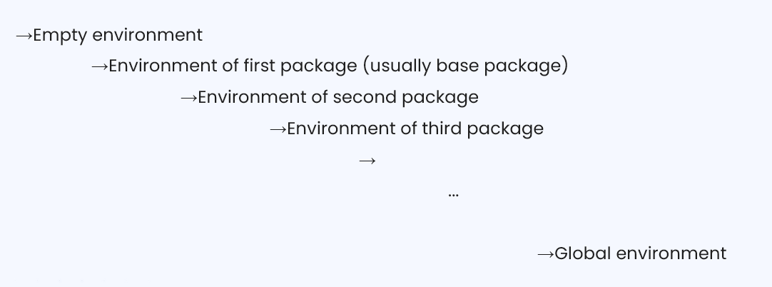
ls()

The parent environment of the global environment is the most recent package that was loaded. Use parent.env(globalenv()) to determine the parent environment.

parent.env(globalenv())

Use ls again to show names in a specific environment.

ls(parent.env(globalenv()))

How R finds a name

When you call a name:

R looks in the current environment’s frame.
If not found, it searches the parent, then the grandparent, and so on.
If still not found, an error occurs.

Environments give context to names, letting you reuse them safely while keeping code manageable.

Example: Finding a name in different environments

max is a function in the base package.

max

## function (..., na.rm = FALSE)  .Primitive("max")

You can create another max in the global environment.

max <- 5
max

## [1] 5

Note that we are NOT replacing the max object in the base environment. We are simply creating ANOTHER object in a different environment. We can still call the original max object in the base environment.

base::max

## function (..., na.rm = FALSE)  .Primitive("max")

Also note that in a particular environment, a name can only be associated with a single object.

Now assigning a new value to the name max in the global environment:

max <- 10

Here, we cannot call the value 5 which was first assigned to the name max in the global environment. But, in a different environment, these names can be bound to different values or objects (e.g. the function max in the base environment).

1.9 Functions as abstractions

In programming, abstraction means hiding the details of how something is done and focusing on what it does. Functions are the main way to achieve this in R.

Why is abstraction important?

There is a term called “don’t repeat yourself” or “DRY” in programming. It suggests that it is a good programming practice to NOT use a block of code, or information, repeatedly.

What we want is to be able to “abstract” this information, i.e., define an object we can call multiple times without having to reveal ALL unnecessary information.

Creating “functions” helps us in abstraction.

Function in R

Note that a function is defined in R with the following syntax:

<NAME OF FUNCTION> <- function(<ARGUMENT 1>, <ARGUMENT 2>, ...){
  <FIRST INSTRUCTION OF THE FUNCTION>
  <SECOND INSTRUCTION OF THE FUNCTION>
  ...
}

This means that the class of <NAME OF FUNCTION> is a function, regardless of the instructions inside it.

Example without abstraction

x <- 1:10
y <- 11:20

mean_x <- sum(x) / length(x)
mean_y <- sum(y) / length(y)

Example WITH abstraction

my_mean <- function(v) {
  sum(v) / length(v)
}

my_mean(1:10)
my_mean(11:20)

## [1] 5.5
## [1] 15.5

The function my_mean() abstracts the process.

We no longer worry about the steps inside—it just “computes the mean.”

R Project and R Markdown

In your devices, open R Studio and create an R project. This shall be your working environment.
Explore how to work with R Markdown.

Visit this link to know more about text formatting and other capabilities of R Markdown:

https://rmarkdown.rstudio.com/authoring_basics.html

Note that for our machine problems, I will be requiring you to use R Markdown for easier documentation. Results must be knitted to HTML or PDF.

Exercise

What is the result?
```
x <- 5
y <- 2
x %/% y + x %% y
```
What is the result?
```
a <- TRUE
b <- FALSE
!a | b
```
What is the result?
```
v <- 1:5
v[v %% 2 == 0]
```
What is the result?
```
x <- c(2, 4, 6)
ifelse(x > 3, x/2, x*2)
```

What does the following code print?

count <- 0
while (count < 3) {
    count <- count + 1
    if (count %% 2 == 0) {
        next
    }
    print(count)
}

What is “abstraction”?
What is the only environment that has no parent environment?
What is the value of x in the global environment after this sequence of codes?
```
x <- 10
update_x <-function(x){
    x <- 20
}
update_x(x)
```

What will be bound to a, b, and x in the global environment after the following program is run?

x <- 3
a <- 5
func <- function(b){
    x <- a + b
        return(x)

}

func(2)

References

- Wickham, H. (2019). Advanced R. Chapman and Hall. https://adv-r.hadley.nz/