CHAPTER 8 Assessing General Diagnostic Plots and Testing for Linearity

In this section, we explore how to assess general diagnostic plots such as Residual Plots, Partial Regression Plots, and Residual Plots. However, graphs can also be used for several other purposes:

• Explore relationships among variables.
• Confirm or negate assumptions.
• Assess the adequacy of a fitted model.
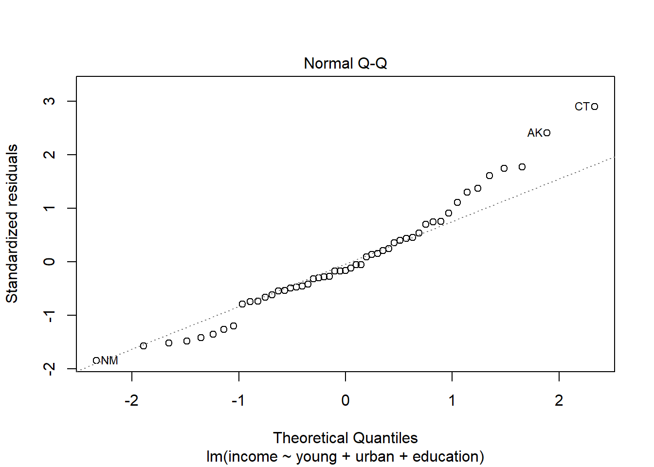
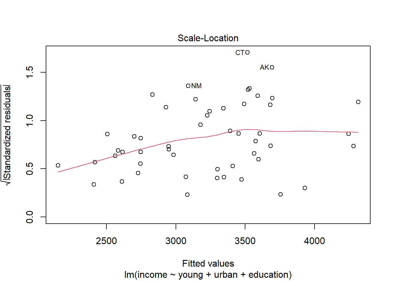
• Detect outlying observations in the data.
• Suggest remedial actions (e.g., transform the data, redesign the experiment, collect more data, etc.).

The assumption of linearity is also checked. If the linearity assumption is not met, some remedial measures are also suggested here.

8.1 Residual Plots

Recall: The residuals of the fitted model is $$\begin{align} \textbf{e} & = \textbf{Y} − \hat{\textbf{Y}}=\textbf{Y} − \textbf{X}\hat{\beta} \\ &= (\textbf{I}-\textbf{X}(\textbf{X}'\textbf{X} )^{−1}\textbf{X}')\textbf{Y}\\ &= (\textbf{I} − \textbf{H})\textbf{Y} \end{align}$$ Review definition and remarks about the residuals in Definition ??

Remarks:

• The residuals is not exactly the error term, but departures from the assumptions of the error terms will likely reflect the residuals.
• To validate assumptions on the error terms, we will validate the assumptions on the residuals instead.
• After we have examined the residuals, we shall be able to conclude either

  1. the assumptions appear to be violated, or

  2. the assumptions do not appear to be violated.

• Concluding (2) does not mean that we are concluding that the assumptions are correct; it means merely that, on the basis of the data we have seen, we have no reason to say that they are incorrect.

Theorem 8.1 (Variance and Covariances of the Residuals)

• $Var(\textbf{e})=\sigma^2(\textbf{I}-\textbf{H})$

• $Var(e_i)=\sigma^2(1-h_{ii})$ where $h_{ii}$ is the $i^{th}$ diagonal element of $\textbf{H}$ (usually called the leverage)

• $Cov(e_i,e_j)=-\sigma^2h_{ij}$

• $\rho(e_i,e_j)=-\frac{h_{ij}}{\sqrt{(1-h_{ii})(1-h_{jj})}}$

Remarks:

• Unlike the error terms $\varepsilon_i$ residuals are not independent to each other and correlation exists among them.
• When the sample size is large in comparison to $p$, this dependence of the residuals has little effect on their use for checking model adequacy.
• The effect is usually negligible. The residuals will be used in validating the assumptions. A simple method of doing this is by looking at the residual plots.

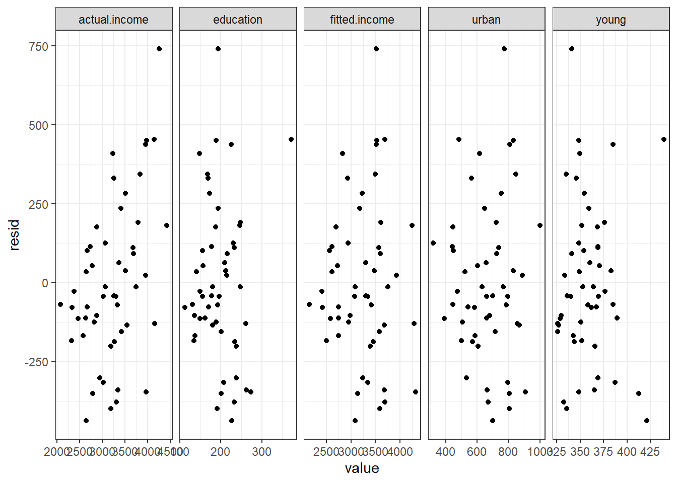
Definition 8.1 (Residual Plot) A residual plot is a scatter plot of the residuals (plotted on the vertical axis of the Cartesian plane) and other elements of regression modelling such as fitted values of Y and values of the regressors $X_j$ (plotted on the horizontal axis).

Why do we plot the residuals against the fitted values and the values of the regressors and NOT against the observed response values for the usual linear model?

• If the model follows all the assumptions, the residuals and the response values are usually correlated.
• But the residuals and regressors and fitted values are not.
  • Theorem ??: $Cov(e_i,X_{ji})=0$
  • Theorem ??: $Cov(e_i,\hat{Y})=0$
• One of our goals in looking at residual plots is to check whether there are patterns in the plot itself.
  • Since the response values and residuals are usually correlated, this relationship will affect the interpretation of the plot, and expected to have some pattern.
  • On the other hand, if there is a recognizable pattern in the residuals vs fitted plot or the residuals vs regressors plot, then there might be something wrong in the model.

library(carData)
library(tidyverse)

## Warning: package 'tidyverse' was built under R version 4.2.3

## Warning: package 'ggplot2' was built under R version 4.2.3

## Warning: package 'tibble' was built under R version 4.2.3

## Warning: package 'tidyr' was built under R version 4.2.3

## Warning: package 'readr' was built under R version 4.2.3

## Warning: package 'purrr' was built under R version 4.2.3

## Warning: package 'dplyr' was built under R version 4.2.3

## Warning: package 'stringr' was built under R version 4.2.3

## Warning: package 'forcats' was built under R version 4.2.3

## Warning: package 'lubridate' was built under R version 4.2.3

## ── Attaching core tidyverse packages ──────────────────────── tidyverse 2.0.0 ──
## ✔ dplyr     1.1.2     ✔ readr     2.1.4
## ✔ forcats   1.0.0     ✔ stringr   1.5.0
## ✔ ggplot2   3.4.2     ✔ tibble    3.2.1
## ✔ lubridate 1.9.2     ✔ tidyr     1.3.0
## ✔ purrr     1.0.1     
## ── Conflicts ────────────────────────────────────────── tidyverse_conflicts() ──
## ✖ dplyr::filter() masks stats::filter()
## ✖ dplyr::lag()    masks stats::lag()
## ℹ Use the conflicted package (<http://conflicted.r-lib.org/>) to force all conflicts to become errors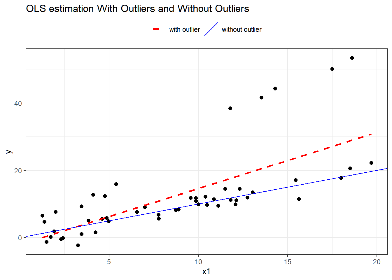

mod_anscombe <- lm(income~young+urban+education, data = Anscombe)
plot(mod_anscombe)

data.frame(resid = resid(mod_anscombe), 
           fitted.income = fitted(mod_anscombe),
           actual.income = Anscombe$income,
           young = Anscombe$young,
           urban = Anscombe$urban,
           education = Anscombe$education) |> 
    pivot_longer(cols = c(actual.income,fitted.income,young,urban,education)) |> 
    ggplot(aes(y = resid, x = value))+
    geom_point()+
    facet_grid(.~name,scales = 'free_x') + theme_bw()

Partial Regression Plots

Partial Residual Plots

8.2 Effects and Usual Causes of Nonlinearity

8.3 Testing for Nonlinearity

8.4 Remedial Measures