6 Gathering and Cleaning Data

6.1 Data gathering

Loading packages

library(readr)
library(dplyr)
library(tidyr)
library(purrr)
library(lubridate)
library(ggplot2)
library(stringr)
library(knitr)
library(xts)
library(zoo)
library(gridExtra)
library(fpp2)
library(RcppRoll)
library(kableExtra)

options(knitr.table.format = "html")

First of all I have to check if I will have the basic data to make the analysis. I need air pollution and weather data of the Gijon area. The town hall of Gijon has an open data web portal here https://transparencia.gijon.es/. We can download pollution air data on csv format from year 2000 to 2017 here:

I downloaded 18 csv files with air pollution and weather data of Gijon from years 2000 to 2017. I saved them in the “data” folder. I downloaded two more files from this web, a csv file with the description of the variables and another csv file with information about the measurement stations.

We take a look to the information included in the stations_info.csv file. It includes the stations addresses, longitude, latitude and their IDs and names. All this information, as we will see, is included in the csv files with pollution and weather data too. So, we are not going to use this file anymore.

stations <- read_delim('data/stations_info.csv',
                       delim = ';',
                       escape_double = FALSE,
                       trim_ws = TRUE,
                       locale = locale(encoding = "ISO-8859-1"),
                       col_types = cols(.default = "c"))
stations

## # A tibble: 6 x 6
##   `"ID;""Título""` `""Dirección""` `""Población""` `""Provincia""`
##   <chr>            <chr>           <chr>           <chr>          
## 1 "\"1;\"\"Consti~ "\"\"Avda. Con~ "\"\"Gijón\"\"" "\"\"Asturias\~
## 2 "\"2;\"\"Argent~ "\"\"Avda. Arg~ "\"\"Gijón\"\"" "\"\"Asturias\~
## 3 "\"3;\"\"H. Fel~ "\"\"H. Felgue~ "\"\"Gijón\"\"" "\"\"Asturias\~
## 4 "\"4;\"\"Castil~ "\"\"Plaza Cas~ "\"\"Gijón\"\"" "\"\"Asturias\~
## 5 "\"10;\"\"Monte~ "\"\"Montevil\~ "\"\"Gijón\"\"" "\"\"Asturias\~
## 6 "\"11;\"\"Santa~ "\"\"Santa Bár~ "\"\"Gijón\"\"" "\"\"Asturias\~
## # ... with 2 more variables: `""latitud""` <chr>, `""longitud""",,` <chr>

We can see on this image the location of each station. http://movil.asturias.es/medioambiente/articulos/ficheros/Informe%20de%20calidad%20del%20aire%20en%20Asturias%202016.pdf

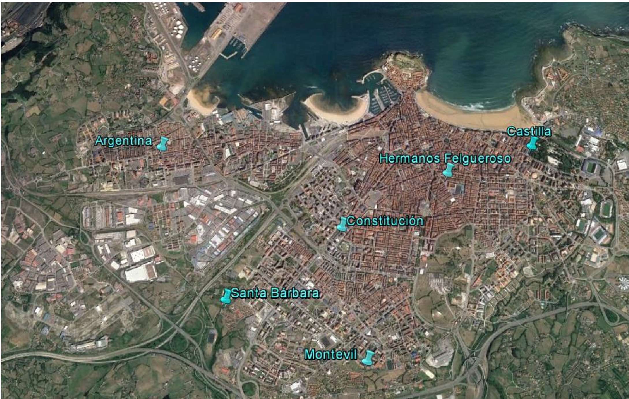
Image source: “Informe de calidad del aire del Principado de Asturias (2016)”.

The air_data_descriptors.csv file contains information about the nature of the elements monitored by the stations. Names, descriptions and units.

variables <- read_csv('data/air_data_descriptors.csv', locale = locale(encoding = "ISO-8859-1"))
variables

## # A tibble: 17 x 4
##    Parametro `Descripción Parámetro`            TAG   Unidad
##    <chr>     <chr>                              <chr> <chr> 
##  1 BEN       Benceno                            BEN   µg/m³ 
##  2 CO        Concentracion de CO                CO    mg/m³ 
##  3 DD        Direccion del viento               DD    Grados
##  4 HR        Humedad relativa                   HR    %hr   
##  5 LL        Precipitacion                      LL    l/m²  
##  6 MXIL      MXileno                            MXIL  µg/m³ 
##  7 NO        Concentracion de NO                NO    µg/m³ 
##  8 NO2       Concentracion de NO2               NO2   µg/m³ 
##  9 O3        Concentracion de Ozono             O3    µg/m³ 
## 10 PM10      Particulas en suspension <10 µg/m³ PM10  µg/m³ 
## 11 PM25      Particulas en Suspension PM 2,5    PM25  µg/m³ 
## 12 PRB       Presion Atmosferica                PRB   mb    
## 13 RS        Radiacion Solar                    RS    W/m²  
## 14 SO2       Concentracion de SO2               SO2   µg/m³ 
## 15 TMP       Temperatura Seca                   TMP   ºC    
## 16 TOL       Tolueno                            TOL   µg/m³ 
## 17 VV        Velocidad del viento               VV    m/s

In order to import the data from the 18 csv files we list all the files in the object data_files.

data_files <- list.files(path = "data", pattern = "air_data_20*")

Then, we map the function read_csv on this list in order to import every file and finally merge them in a unique dataframe (air_data_0) with reduce(rbind).

air_data_0 <- data_files %>%
    map(function(x) {
        read_csv(paste0("./data/", x), locale = locale(encoding = "ISO-8859-1"), col_types = cols(.default = "c"))
    }) %>%
    reduce(rbind)

We take a look to the dataset

glimpse(air_data_0)

## Observations: 722,774
## Variables: 22
## $ Estación            <chr> "1", "1", "1", "1", "1", "1", "1", "1", "1...
## $ Título              <chr> "Estación Avenida Constitución", "Estación...
## $ latitud             <chr> "43.529806", "43.529806", "43.529806", "43...
## $ longitud            <chr> "-5.673428", "-5.673428", "-5.673428", "-5...
## $ `Fecha Solar (UTC)` <chr> "2000-01-01T00:00:00", "2000-01-01T01:00:0...
## $ SO2                 <chr> "23", "29", "40", "50", "39", "39", "40", ...
## $ NO                  <chr> "89", "73", "53", "46", "35", "26", "27", ...
## $ NO2                 <chr> "65", "60", "57", "53", "50", "49", "51", ...
## $ CO                  <chr> "1.97", "1.61", "1.13", "1.06", "0.95", "0...
## $ PM10                <chr> "53", "63", "56", "58", "50", "50", "57", ...
## $ O3                  <chr> "9", "8", "7", "5", "6", "7", "7", "4", "5...
## $ dd                  <chr> "245", "222", "228", "239", "244", "218", ...
## $ vv                  <chr> "0.34", "1.06", "0.71", "0.84", "0.89", "0...
## $ TMP                 <chr> "5.7", "5.4", "5.3", "5.1", "4.6", "4.6", ...
## $ HR                  <chr> "76", "73", "72", "71", "72", "69", "68", ...
## $ PRB                 <chr> "1026", "1025", "1025", "1025", "1024", "1...
## $ RS                  <chr> "33", "33", "33", "33", "33", "33", "33", ...
## $ LL                  <chr> "0", "0", "0", "0", "0", "0", "0", "0", "0...
## $ BEN                 <chr> NA, NA, NA, NA, NA, NA, NA, NA, NA, NA, NA...
## $ TOL                 <chr> NA, NA, NA, NA, NA, NA, NA, NA, NA, NA, NA...
## $ MXIL                <chr> NA, NA, NA, NA, NA, NA, NA, NA, NA, NA, NA...
## $ PM25                <chr> NA, NA, NA, NA, NA, NA, NA, NA, NA, NA, NA...

We change some variables names.

# Variables names changing
air_data_1 <- air_data_0 %>% rename(station = 'Estación',
                                    station_name = 'Título',
                                    date_time_utc = 'Fecha Solar (UTC)',
                                    latitude = latitud,
                                    longitude = longitud,
                                    wd = dd,
                                    ws = vv)

6.2 Data cleaning

We imported all the columns as characters in order to avoid problems with the format attributions. So, we have to make now some format variable changes.

We change the date_time_utc format from character to date time.

air_data_1$date_time_utc <- ymd_hms(air_data_1$date_time_utc)

We change the station and station_name formats from character to factor.

air_data_1$station <- as.factor(air_data_1$station)
air_data_1$station_name <- as.factor(air_data_1$station_name)

We create a vector with all the variables we want to be numeric

num <- colnames(air_data_1)[c(3, 4, 6:22)]

We make the conversion of this set of variables to numeric

air_data_1 <- air_data_1 %>% mutate_at(num, as.numeric)

We create a dictionary with an alias for each station in order to add a new variable with more convenient station names

alias_dict <- data.frame(
      station = c("1", "2", "3", "4", "10", "11"),
      station_alias = c("Constitucion", "Argentina", "H. Felgueroso", "Castilla", "Montevil", "Santa Barbara")
)

We join the alias dictionary to the air_data_1 data frame to add the new variable to the data set.

air_data_1 <- air_data_1 %>% left_join(alias_dict, by = 'station')

We call the summary function to inspect the data main indicators

summary(air_data_1)

##  station                                   station_name       latitude    
##  1 :157727   Estación Avenida Argentina          :157798   Min.   :43.52  
##  10: 74630   Estación Avenida Castilla           :157409   1st Qu.:43.53  
##  11: 17544   Estación Avenida Constitución       :157727   Median :43.54  
##  2 :157798   Estación Avenida Hermanos Felgueroso:157666   Mean   :43.53  
##  3 :157666   Estación de Montevil                : 74630   3rd Qu.:43.54  
##  4 :157409   Estación Santa Bárbara              : 17544   Max.   :43.54  
##                                                                           
##    longitude      date_time_utc                      SO2          
##  Min.   :-5.699   Min.   :2000-01-01 00:00:00   Min.   :-9999.00  
##  1st Qu.:-5.673   1st Qu.:2005-02-25 05:00:00   1st Qu.:    4.00  
##  Median :-5.672   Median :2010-02-23 11:00:00   Median :    6.00  
##  Mean   :-5.670   Mean   :2009-09-06 07:33:13   Mean   :    9.77  
##  3rd Qu.:-5.658   3rd Qu.:2014-04-09 06:00:00   3rd Qu.:   11.00  
##  Max.   :-5.646   Max.   :2018-01-01 00:00:00   Max.   : 2662.00  
##                                                 NA's   :33742     
##        NO                NO2                 CO             PM10         
##  Min.   :-9999.00   Min.   :-9999.00   Min.   : 0.00   Min.   :-9999.00  
##  1st Qu.:    4.40   1st Qu.:   16.00   1st Qu.: 0.22   1st Qu.:   19.00  
##  Median :   10.00   Median :   28.00   Median : 0.36   Median :   30.00  
##  Mean   :   21.37   Mean   :   32.04   Mean   : 0.49   Mean   :   35.88  
##  3rd Qu.:   23.00   3rd Qu.:   45.00   3rd Qu.: 0.59   3rd Qu.:   46.00  
##  Max.   : 1248.00   Max.   : 1003.20   Max.   :58.20   Max.   : 1000.00  
##  NA's   :16989      NA's   :16446      NA's   :90390   NA's   :88598     
##        O3                 wd               ws              TMP        
##  Min.   :-9999.00   Min.   :  0.0    Min.   : 0.0     Min.   :-40.0   
##  1st Qu.:   17.00   1st Qu.: 96.0    1st Qu.: 0.2     1st Qu.: 10.9   
##  Median :   37.00   Median :159.0    Median : 0.7     Median : 14.7   
##  Mean   :   38.97   Mean   :161.8    Mean   : 1.0     Mean   : 14.6   
##  3rd Qu.:   57.00   3rd Qu.:228.0    3rd Qu.: 1.5     3rd Qu.: 18.4   
##  Max.   :  998.00   Max.   :360.0    Max.   :29.8     Max.   : 47.4   
##  NA's   :31417      NA's   :494134   NA's   :493893   NA's   :494151  
##        HR              PRB               RS               LL        
##  Min.   :  0.0    Min.   : 800     Min.   :  -1.0   Min.   : 0.0    
##  1st Qu.: 69.0    1st Qu.:1007     1st Qu.:  17.0   1st Qu.: 0.0    
##  Median : 80.0    Median :1013     Median :  46.0   Median : 0.0    
##  Mean   : 78.3    Mean   :1012     Mean   : 125.2   Mean   : 0.1    
##  3rd Qu.: 89.0    3rd Qu.:1018     3rd Qu.: 149.0   3rd Qu.: 0.0    
##  Max.   :123.0    Max.   :1282     Max.   :1470.0   Max.   :24.6    
##  NA's   :494176   NA's   :494019   NA's   :494273   NA's   :494124  
##       BEN              TOL              MXIL             PM25       
##  Min.   : 0.0     Min.   : -0.2    Min.   : -0.3    Min.   :  0.0   
##  1st Qu.: 0.1     1st Qu.:  0.4    1st Qu.:  0.2    1st Qu.:  5.0   
##  Median : 0.3     Median :  1.0    Median :  0.3    Median :  9.0   
##  Mean   : 0.5     Mean   :  2.5    Mean   :  1.3    Mean   : 11.3   
##  3rd Qu.: 0.5     3rd Qu.:  2.5    3rd Qu.:  0.9    3rd Qu.: 15.0   
##  Max.   :22.5     Max.   :196.0    Max.   :220.0    Max.   :947.0   
##  NA's   :629358   NA's   :629380   NA's   :635123   NA's   :554185  
##        station_alias   
##  Argentina    :157798  
##  Castilla     :157409  
##  Constitucion :157727  
##  H. Felgueroso:157666  
##  Montevil     : 74630  
##  Santa Barbara: 17544  
## 

There are several variables which minimun values are -9999.

kable(air_data_1 %>% filter(SO2 == -9999 |
                              NO == -9999 |
                              NO2 == -9999 |
                              PM10 == -9999 |
                              O3 == -9999 )) %>%
                              kable_styling()

station	station_name	latitude	longitude	date_time_utc	SO2	NO	NO2	CO	PM10	O3	wd	ws	TMP	HR	PRB	RS	LL	BEN	TOL	MXIL	PM25	station_alias
3	Estación Avenida Hermanos Felgueroso	43.53506	-5.658123	2000-01-27 00:00:00	-9999	-9999	-9999	0	-9999	-9999	NA	NA	NA	NA	NA	NA	NA	NA	NA	NA	NA	H. Felgueroso
3	Estación Avenida Hermanos Felgueroso	43.53506	-5.658123	2000-01-27 01:00:00	-9999	-9999	-9999	0	-9999	-9999	NA	NA	NA	NA	NA	NA	NA	NA	NA	NA	NA	H. Felgueroso
3	Estación Avenida Hermanos Felgueroso	43.53506	-5.658123	2000-01-27 02:00:00	-9999	-9999	-9999	0	-9999	-9999	NA	NA	NA	NA	NA	NA	NA	NA	NA	NA	NA	H. Felgueroso
3	Estación Avenida Hermanos Felgueroso	43.53506	-5.658123	2000-01-27 03:00:00	-9999	-9999	-9999	0	-9999	-9999	NA	NA	NA	NA	NA	NA	NA	NA	NA	NA	NA	H. Felgueroso
3	Estación Avenida Hermanos Felgueroso	43.53506	-5.658123	2000-01-27 04:00:00	-9999	-9999	-9999	0	-9999	-9999	NA	NA	NA	NA	NA	NA	NA	NA	NA	NA	NA	H. Felgueroso
3	Estación Avenida Hermanos Felgueroso	43.53506	-5.658123	2000-01-27 05:00:00	-9999	-9999	-9999	0	-9999	-9999	NA	NA	NA	NA	NA	NA	NA	NA	NA	NA	NA	H. Felgueroso
3	Estación Avenida Hermanos Felgueroso	43.53506	-5.658123	2000-01-27 06:00:00	-9999	-9999	-9999	0	-9999	-9999	NA	NA	NA	NA	NA	NA	NA	NA	NA	NA	NA	H. Felgueroso
3	Estación Avenida Hermanos Felgueroso	43.53506	-5.658123	2000-01-27 07:00:00	-9999	-9999	-9999	0	-9999	-9999	NA	NA	NA	NA	NA	NA	NA	NA	NA	NA	NA	H. Felgueroso
3	Estación Avenida Hermanos Felgueroso	43.53506	-5.658123	2000-01-27 08:00:00	-9999	-9999	-9999	0	-9999	-9999	NA	NA	NA	NA	NA	NA	NA	NA	NA	NA	NA	H. Felgueroso
3	Estación Avenida Hermanos Felgueroso	43.53506	-5.658123	2000-01-27 09:00:00	-9999	-9999	-9999	0	-9999	-9999	NA	NA	NA	NA	NA	NA	NA	NA	NA	NA	NA	H. Felgueroso
3	Estación Avenida Hermanos Felgueroso	43.53506	-5.658123	2000-01-27 10:00:00	-9999	-9999	-9999	0	-9999	-9999	NA	NA	NA	NA	NA	NA	NA	NA	NA	NA	NA	H. Felgueroso
3	Estación Avenida Hermanos Felgueroso	43.53506	-5.658123	2000-01-27 11:00:00	-9999	-9999	-9999	0	-9999	-9999	NA	NA	NA	NA	NA	NA	NA	NA	NA	NA	NA	H. Felgueroso
3	Estación Avenida Hermanos Felgueroso	43.53506	-5.658123	2000-01-27 12:00:00	-9999	-9999	-9999	0	-9999	-9999	NA	NA	NA	NA	NA	NA	NA	NA	NA	NA	NA	H. Felgueroso
3	Estación Avenida Hermanos Felgueroso	43.53506	-5.658123	2000-01-27 13:00:00	-9999	-9999	-9999	0	-9999	-9999	NA	NA	NA	NA	NA	NA	NA	NA	NA	NA	NA	H. Felgueroso
3	Estación Avenida Hermanos Felgueroso	43.53506	-5.658123	2000-01-27 14:00:00	-9999	-9999	-9999	0	-9999	-9999	NA	NA	NA	NA	NA	NA	NA	NA	NA	NA	NA	H. Felgueroso
3	Estación Avenida Hermanos Felgueroso	43.53506	-5.658123	2000-01-27 15:00:00	-9999	-9999	-9999	0	-9999	-9999	NA	NA	NA	NA	NA	NA	NA	NA	NA	NA	NA	H. Felgueroso
3	Estación Avenida Hermanos Felgueroso	43.53506	-5.658123	2000-01-27 16:00:00	-9999	-9999	-9999	0	-9999	-9999	NA	NA	NA	NA	NA	NA	NA	NA	NA	NA	NA	H. Felgueroso
3	Estación Avenida Hermanos Felgueroso	43.53506	-5.658123	2000-01-27 17:00:00	-9999	-9999	-9999	0	-9999	-9999	NA	NA	NA	NA	NA	NA	NA	NA	NA	NA	NA	H. Felgueroso
3	Estación Avenida Hermanos Felgueroso	43.53506	-5.658123	2000-01-27 18:00:00	-9999	-9999	-9999	0	-9999	-9999	NA	NA	NA	NA	NA	NA	NA	NA	NA	NA	NA	H. Felgueroso
3	Estación Avenida Hermanos Felgueroso	43.53506	-5.658123	2000-01-27 19:00:00	-9999	-9999	-9999	0	-9999	-9999	NA	NA	NA	NA	NA	NA	NA	NA	NA	NA	NA	H. Felgueroso
3	Estación Avenida Hermanos Felgueroso	43.53506	-5.658123	2000-01-27 20:00:00	-9999	-9999	-9999	0	-9999	-9999	NA	NA	NA	NA	NA	NA	NA	NA	NA	NA	NA	H. Felgueroso
3	Estación Avenida Hermanos Felgueroso	43.53506	-5.658123	2000-01-27 21:00:00	-9999	-9999	-9999	0	-9999	-9999	NA	NA	NA	NA	NA	NA	NA	NA	NA	NA	NA	H. Felgueroso
3	Estación Avenida Hermanos Felgueroso	43.53506	-5.658123	2000-01-27 22:00:00	-9999	-9999	-9999	0	-9999	-9999	NA	NA	NA	NA	NA	NA	NA	NA	NA	NA	NA	H. Felgueroso
3	Estación Avenida Hermanos Felgueroso	43.53506	-5.658123	2000-01-27 23:00:00	-9999	-9999	-9999	0	-9999	-9999	NA	NA	NA	NA	NA	NA	NA	NA	NA	NA	NA	H. Felgueroso

They are all from the same day (2000-01-27) and from the same station (‘H. Felgueroso’). We replace these values by NAs.

air_data_2 <- air_data_1 %>% mutate(SO2 = replace(SO2, SO2 == -9999, NA),
                                    NO = replace(NO, NO == -9999, NA),
                                    NO2 = replace(NO2, NO2 == -9999, NA),
                                    PM10 = replace(PM10, PM10 == -9999, NA),
                                    O3 = replace(O3, O3 == -9999, NA))

We check again the output of the summary function.

summary(air_data_2)

##  station                                   station_name       latitude    
##  1 :157727   Estación Avenida Argentina          :157798   Min.   :43.52  
##  10: 74630   Estación Avenida Castilla           :157409   1st Qu.:43.53  
##  11: 17544   Estación Avenida Constitución       :157727   Median :43.54  
##  2 :157798   Estación Avenida Hermanos Felgueroso:157666   Mean   :43.53  
##  3 :157666   Estación de Montevil                : 74630   3rd Qu.:43.54  
##  4 :157409   Estación Santa Bárbara              : 17544   Max.   :43.54  
##                                                                           
##    longitude      date_time_utc                      SO2         
##  Min.   :-5.699   Min.   :2000-01-01 00:00:00   Min.   :  -2.00  
##  1st Qu.:-5.673   1st Qu.:2005-02-25 05:00:00   1st Qu.:   4.00  
##  Median :-5.672   Median :2010-02-23 11:00:00   Median :   6.00  
##  Mean   :-5.670   Mean   :2009-09-06 07:33:13   Mean   :  10.12  
##  3rd Qu.:-5.658   3rd Qu.:2014-04-09 06:00:00   3rd Qu.:  11.00  
##  Max.   :-5.646   Max.   :2018-01-01 00:00:00   Max.   :2662.00  
##                                                 NA's   :33766    
##        NO               NO2                CO             PM10        
##  Min.   :   0.00   Min.   :   0.00   Min.   : 0.00   Min.   :   0.00  
##  1st Qu.:   4.40   1st Qu.:  16.00   1st Qu.: 0.22   1st Qu.:  19.00  
##  Median :  10.00   Median :  28.00   Median : 0.36   Median :  30.00  
##  Mean   :  21.71   Mean   :  32.38   Mean   : 0.49   Mean   :  36.26  
##  3rd Qu.:  23.00   3rd Qu.:  45.00   3rd Qu.: 0.59   3rd Qu.:  46.00  
##  Max.   :1248.00   Max.   :1003.20   Max.   :58.20   Max.   :1000.00  
##  NA's   :17013     NA's   :16470     NA's   :90390   NA's   :88622    
##        O3               wd               ws              TMP        
##  Min.   :  0.00   Min.   :  0.0    Min.   : 0.0     Min.   :-40.0   
##  1st Qu.: 17.00   1st Qu.: 96.0    1st Qu.: 0.2     1st Qu.: 10.9   
##  Median : 37.00   Median :159.0    Median : 0.7     Median : 14.7   
##  Mean   : 39.32   Mean   :161.8    Mean   : 1.0     Mean   : 14.6   
##  3rd Qu.: 57.00   3rd Qu.:228.0    3rd Qu.: 1.5     3rd Qu.: 18.4   
##  Max.   :998.00   Max.   :360.0    Max.   :29.8     Max.   : 47.4   
##  NA's   :31441    NA's   :494134   NA's   :493893   NA's   :494151  
##        HR              PRB               RS               LL        
##  Min.   :  0.0    Min.   : 800     Min.   :  -1.0   Min.   : 0.0    
##  1st Qu.: 69.0    1st Qu.:1007     1st Qu.:  17.0   1st Qu.: 0.0    
##  Median : 80.0    Median :1013     Median :  46.0   Median : 0.0    
##  Mean   : 78.3    Mean   :1012     Mean   : 125.2   Mean   : 0.1    
##  3rd Qu.: 89.0    3rd Qu.:1018     3rd Qu.: 149.0   3rd Qu.: 0.0    
##  Max.   :123.0    Max.   :1282     Max.   :1470.0   Max.   :24.6    
##  NA's   :494176   NA's   :494019   NA's   :494273   NA's   :494124  
##       BEN              TOL              MXIL             PM25       
##  Min.   : 0.0     Min.   : -0.2    Min.   : -0.3    Min.   :  0.0   
##  1st Qu.: 0.1     1st Qu.:  0.4    1st Qu.:  0.2    1st Qu.:  5.0   
##  Median : 0.3     Median :  1.0    Median :  0.3    Median :  9.0   
##  Mean   : 0.5     Mean   :  2.5    Mean   :  1.3    Mean   : 11.3   
##  3rd Qu.: 0.5     3rd Qu.:  2.5    3rd Qu.:  0.9    3rd Qu.: 15.0   
##  Max.   :22.5     Max.   :196.0    Max.   :220.0    Max.   :947.0   
##  NA's   :629358   NA's   :629380   NA's   :635123   NA's   :554185  
##        station_alias   
##  Argentina    :157798  
##  Castilla     :157409  
##  Constitucion :157727  
##  H. Felgueroso:157666  
##  Montevil     : 74630  
##  Santa Barbara: 17544  
## 

Some pollutant variables have as minimum negative values. It does not make much sense. We take a look to the data in order to quantify the problem.

30 SO2 observations between 2015-12-25 and 2015-12-28 from the Montevil station:

(neg_SO2 <- air_data_2 %>% filter(SO2 < 0) %>%
                          summarise(n = n()))

## # A tibble: 1 x 1
##       n
##   <int>
## 1    30

2 RS observations from the Constitucion station:

(neg_RS <- air_data_2 %>% filter(RS < 0) %>%
                          summarise(n = n()))

## # A tibble: 1 x 1
##       n
##   <int>
## 1     2

27 TOL observations between the 2008-12-11 and the 2008-12-15 from the Constitucion station:

(neg_TOL <- air_data_2 %>% filter(TOL < 0) %>%
                          summarise(n = n()))

## # A tibble: 1 x 1
##       n
##   <int>
## 1    27

59 MXIL observations between the 2008-12-10 and the 2008-12-15 from the Constitucion station:

(neg_MXIL <- air_data_2 %>% filter(MXIL < 0) %>%
                          summarise(n = n()))

## # A tibble: 1 x 1
##       n
##   <int>
## 1    59

There are not many cases. We replace them all by NAs and call again the summary function.

air_data_2 <- air_data_2 %>% mutate(SO2 = replace(SO2, SO2 < 0, NA),
                                    RS = replace(RS, RS < 0, NA),
                                    TOL = replace(TOL, TOL < 0, NA),
                                    MXIL = replace(MXIL, MXIL < 0, NA))

summary(air_data_2)

##  station                                   station_name       latitude    
##  1 :157727   Estación Avenida Argentina          :157798   Min.   :43.52  
##  10: 74630   Estación Avenida Castilla           :157409   1st Qu.:43.53  
##  11: 17544   Estación Avenida Constitución       :157727   Median :43.54  
##  2 :157798   Estación Avenida Hermanos Felgueroso:157666   Mean   :43.53  
##  3 :157666   Estación de Montevil                : 74630   3rd Qu.:43.54  
##  4 :157409   Estación Santa Bárbara              : 17544   Max.   :43.54  
##                                                                           
##    longitude      date_time_utc                      SO2         
##  Min.   :-5.699   Min.   :2000-01-01 00:00:00   Min.   :   0.00  
##  1st Qu.:-5.673   1st Qu.:2005-02-25 05:00:00   1st Qu.:   4.00  
##  Median :-5.672   Median :2010-02-23 11:00:00   Median :   6.00  
##  Mean   :-5.670   Mean   :2009-09-06 07:33:13   Mean   :  10.12  
##  3rd Qu.:-5.658   3rd Qu.:2014-04-09 06:00:00   3rd Qu.:  11.00  
##  Max.   :-5.646   Max.   :2018-01-01 00:00:00   Max.   :2662.00  
##                                                 NA's   :33796    
##        NO               NO2                CO             PM10        
##  Min.   :   0.00   Min.   :   0.00   Min.   : 0.00   Min.   :   0.00  
##  1st Qu.:   4.40   1st Qu.:  16.00   1st Qu.: 0.22   1st Qu.:  19.00  
##  Median :  10.00   Median :  28.00   Median : 0.36   Median :  30.00  
##  Mean   :  21.71   Mean   :  32.38   Mean   : 0.49   Mean   :  36.26  
##  3rd Qu.:  23.00   3rd Qu.:  45.00   3rd Qu.: 0.59   3rd Qu.:  46.00  
##  Max.   :1248.00   Max.   :1003.20   Max.   :58.20   Max.   :1000.00  
##  NA's   :17013     NA's   :16470     NA's   :90390   NA's   :88622    
##        O3               wd               ws              TMP        
##  Min.   :  0.00   Min.   :  0.0    Min.   : 0.0     Min.   :-40.0   
##  1st Qu.: 17.00   1st Qu.: 96.0    1st Qu.: 0.2     1st Qu.: 10.9   
##  Median : 37.00   Median :159.0    Median : 0.7     Median : 14.7   
##  Mean   : 39.32   Mean   :161.8    Mean   : 1.0     Mean   : 14.6   
##  3rd Qu.: 57.00   3rd Qu.:228.0    3rd Qu.: 1.5     3rd Qu.: 18.4   
##  Max.   :998.00   Max.   :360.0    Max.   :29.8     Max.   : 47.4   
##  NA's   :31441    NA's   :494134   NA's   :493893   NA's   :494151  
##        HR              PRB               RS               LL        
##  Min.   :  0.0    Min.   : 800     Min.   :   0.0   Min.   : 0.0    
##  1st Qu.: 69.0    1st Qu.:1007     1st Qu.:  17.0   1st Qu.: 0.0    
##  Median : 80.0    Median :1013     Median :  46.0   Median : 0.0    
##  Mean   : 78.3    Mean   :1012     Mean   : 125.2   Mean   : 0.1    
##  3rd Qu.: 89.0    3rd Qu.:1018     3rd Qu.: 149.0   3rd Qu.: 0.0    
##  Max.   :123.0    Max.   :1282     Max.   :1470.0   Max.   :24.6    
##  NA's   :494176   NA's   :494019   NA's   :494275   NA's   :494124  
##       BEN              TOL              MXIL             PM25       
##  Min.   : 0.0     Min.   :  0.0    Min.   :  0.0    Min.   :  0.0   
##  1st Qu.: 0.1     1st Qu.:  0.4    1st Qu.:  0.2    1st Qu.:  5.0   
##  Median : 0.3     Median :  1.0    Median :  0.3    Median :  9.0   
##  Mean   : 0.5     Mean   :  2.5    Mean   :  1.3    Mean   : 11.3   
##  3rd Qu.: 0.5     3rd Qu.:  2.5    3rd Qu.:  0.9    3rd Qu.: 15.0   
##  Max.   :22.5     Max.   :196.0    Max.   :220.0    Max.   :947.0   
##  NA's   :629358   NA's   :629407   NA's   :635182   NA's   :554185  
##        station_alias   
##  Argentina    :157798  
##  Castilla     :157409  
##  Constitucion :157727  
##  H. Felgueroso:157666  
##  Montevil     : 74630  
##  Santa Barbara: 17544  
## 

We take a look to the data completeness. What proportion of nas do we have by variable, station, year, etc?

data_completeness <- air_data_2 %>%
  group_by(station_alias, year = year(date_time_utc)) %>%
  summarise_all(funs(round(sum(!is.na(.))/n(), 2))) %>% # We obtain the proportion of 'not NAs'
  select(-c(3:7, 25:28)) # These columns do not have any na. We exclude them.

head(data_completeness, 10) %>%
  kable() %>%
  kable_styling()

station_alias	year	SO2	NO	NO2	CO	PM10	O3	wd	ws	TMP	HR	PRB	RS	LL	BEN	TOL	MXIL	PM25
Argentina	2000	0.99	0.97	0.97	0.96	0.94	0.97	0	0	0	0	0	0	0	0	0	0	0
Argentina	2001	0.99	0.99	0.99	0.98	0.97	0.99	0	0	0	0	0	0	0	0	0	0	0
Argentina	2002	1.00	0.99	0.99	0.99	0.99	1.00	0	0	0	0	0	0	0	0	0	0	0
Argentina	2003	0.99	0.98	0.98	0.98	0.99	0.99	0	0	0	0	0	0	0	0	0	0	0
Argentina	2004	0.98	0.96	0.97	0.99	1.00	1.00	0	0	0	0	0	0	0	0	0	0	0
Argentina	2005	0.98	0.96	0.98	1.00	1.00	1.00	0	0	0	0	0	0	0	0	0	0	0
Argentina	2006	0.92	0.90	0.92	0.92	0.93	0.93	0	0	0	0	0	0	0	0	0	0	0
Argentina	2007	0.98	0.99	0.99	0.98	0.99	0.99	0	0	0	0	0	0	0	0	0	0	0
Argentina	2008	0.98	0.96	0.98	0.97	0.98	0.98	0	0	0	0	0	0	0	0	0	0	0
Argentina	2009	1.00	1.00	1.00	0.98	1.00	1.00	0	0	0	0	0	0	0	0	0	0	0

We are going to check the data completeness by station:

Constitución: There is data registered from the variables SO2, NO, NO2, CO, PM10, 03, dd, vv, TMP, HR, PRB, HS and LL since the year 2000. There are measurements of the variables BEN, TOL and MXIL since the year 2006 (only 0.01% ). The PM25 particles are monitored since the year 2008 (2008: only covered 0,02% of the year). During the year 2008 the completeness of several variables (HR, PRB, HS, LL, BEN, TOL y MXIL) decrease until 88% (to do: check there was not caused by a data importing problem.)

constitucion_data <- data_completeness %>% filter(station_alias == 'Constitucion')
constitucion_data %>%
                  kable() %>%
                  kable_styling()

station_alias	year	SO2	NO	NO2	CO	PM10	O3	wd	ws	TMP	HR	PRB	RS	LL	BEN	TOL	MXIL	PM25
Constitucion	2000	0.97	0.95	0.95	0.97	0.92	0.93	0.96	0.98	0.96	0.95	0.97	0.95	0.96	0.00	0.00	0.00	0.00
Constitucion	2001	0.99	0.99	0.99	0.98	0.99	0.99	1.00	1.00	1.00	0.99	1.00	1.00	1.00	0.00	0.00	0.00	0.00
Constitucion	2002	1.00	1.00	1.00	0.99	0.99	0.99	1.00	1.00	1.00	1.00	1.00	1.00	1.00	0.00	0.00	0.00	0.00
Constitucion	2003	0.99	0.99	0.99	0.98	0.99	0.99	0.99	0.99	0.99	0.99	0.99	0.99	0.99	0.00	0.00	0.00	0.00
Constitucion	2004	0.99	0.99	0.99	0.99	0.99	1.00	1.00	1.00	1.00	1.00	1.00	1.00	1.00	0.00	0.00	0.00	0.00
Constitucion	2005	0.98	0.99	0.99	0.99	0.99	0.99	0.99	0.99	0.99	0.99	0.99	0.99	0.99	0.00	0.00	0.00	0.00
Constitucion	2006	0.91	0.91	0.91	0.90	0.91	0.91	0.91	0.91	0.91	0.91	0.91	0.91	0.91	0.01	0.01	0.01	0.00
Constitucion	2007	0.98	0.99	0.99	0.97	0.99	0.99	0.99	0.99	0.99	0.99	0.99	0.99	0.99	0.99	0.99	0.99	0.00
Constitucion	2008	0.98	0.99	0.99	0.99	0.99	1.00	0.88	0.88	0.88	0.88	0.88	0.88	0.88	0.88	0.88	0.88	0.02
Constitucion	2009	0.99	0.99	0.99	0.99	1.00	1.00	1.00	1.00	1.00	1.00	1.00	1.00	1.00	1.00	1.00	1.00	1.00
Constitucion	2010	0.99	0.99	0.99	0.99	0.99	0.99	1.00	1.00	1.00	1.00	1.00	1.00	1.00	0.99	0.99	0.99	0.99
Constitucion	2011	0.99	0.99	0.99	0.99	0.99	0.99	0.99	0.99	0.99	0.99	0.99	0.99	0.99	0.98	0.98	0.98	0.99
Constitucion	2012	0.97	0.97	0.97	0.96	0.97	0.96	0.97	0.97	0.97	0.97	0.97	0.97	0.97	0.96	0.96	0.96	0.97
Constitucion	2013	0.99	0.99	0.99	0.99	1.00	0.99	1.00	1.00	1.00	1.00	1.00	1.00	1.00	0.99	0.99	0.99	1.00
Constitucion	2014	1.00	1.00	1.00	1.00	1.00	1.00	1.00	1.00	1.00	1.00	1.00	1.00	1.00	0.99	0.99	0.99	1.00
Constitucion	2015	0.98	0.98	0.98	0.98	0.99	0.98	0.99	0.99	0.99	0.99	0.99	0.99	0.99	0.98	0.98	0.32	0.98
Constitucion	2016	0.95	0.95	0.95	0.95	0.95	0.95	0.98	0.98	0.97	0.97	0.97	0.97	0.97	0.90	0.90	0.90	0.95
Constitucion	2017	0.99	0.99	0.99	0.99	1.00	0.99	1.00	1.00	1.00	1.00	1.00	1.00	1.00	0.99	0.99	0.99	1.00
Constitucion	2018	1.00	1.00	1.00	1.00	1.00	1.00	1.00	1.00	1.00	1.00	1.00	1.00	1.00	1.00	1.00	1.00	1.00

Argentina: data since the year 2000. Variables: SO2, NO, NO2, CO, PM10 and 03.

argentina_data <- data_completeness %>% filter(station_alias == 'Argentina')
argentina_data %>%
            kable() %>%
            kable_styling()

station_alias	year	SO2	NO	NO2	CO	PM10	O3	wd	ws	TMP	HR	PRB	RS	LL	BEN	TOL	MXIL	PM25
Argentina	2000	0.99	0.97	0.97	0.96	0.94	0.97	0	0	0	0	0	0	0	0	0	0	0
Argentina	2001	0.99	0.99	0.99	0.98	0.97	0.99	0	0	0	0	0	0	0	0	0	0	0
Argentina	2002	1.00	0.99	0.99	0.99	0.99	1.00	0	0	0	0	0	0	0	0	0	0	0
Argentina	2003	0.99	0.98	0.98	0.98	0.99	0.99	0	0	0	0	0	0	0	0	0	0	0
Argentina	2004	0.98	0.96	0.97	0.99	1.00	1.00	0	0	0	0	0	0	0	0	0	0	0
Argentina	2005	0.98	0.96	0.98	1.00	1.00	1.00	0	0	0	0	0	0	0	0	0	0	0
Argentina	2006	0.92	0.90	0.92	0.92	0.93	0.93	0	0	0	0	0	0	0	0	0	0	0
Argentina	2007	0.98	0.99	0.99	0.98	0.99	0.99	0	0	0	0	0	0	0	0	0	0	0
Argentina	2008	0.98	0.96	0.98	0.97	0.98	0.98	0	0	0	0	0	0	0	0	0	0	0
Argentina	2009	1.00	1.00	1.00	0.98	1.00	1.00	0	0	0	0	0	0	0	0	0	0	0
Argentina	2010	0.99	0.99	1.00	0.99	1.00	1.00	0	0	0	0	0	0	0	0	0	0	0
Argentina	2011	0.98	0.99	0.99	0.98	0.99	0.99	0	0	0	0	0	0	0	0	0	0	0
Argentina	2012	0.99	0.96	0.96	0.96	1.00	1.00	0	0	0	0	0	0	0	0	0	0	0
Argentina	2013	0.99	0.99	0.99	0.99	1.00	0.99	0	0	0	0	0	0	0	0	0	0	0
Argentina	2014	1.00	0.99	0.99	1.00	1.00	1.00	0	0	0	0	0	0	0	0	0	0	0
Argentina	2015	0.99	0.99	0.99	0.99	0.99	0.99	0	0	0	0	0	0	0	0	0	0	0
Argentina	2016	0.99	0.99	0.99	0.99	0.99	0.99	0	0	0	0	0	0	0	0	0	0	0
Argentina	2017	0.99	0.99	0.99	0.99	0.99	0.99	0	0	0	0	0	0	0	0	0	0	0
Argentina	2018	1.00	1.00	1.00	1.00	1.00	1.00	0	0	0	0	0	0	0	0	0	0	0

H. Felgueroso: data since the year 2000. Variables: SO2, NO, NO2, CO, PM10 and 03. During the year 2006 the completeness of the data decrease until 88% (to do: check there was not caused by a data importing problem.)

felgueroso_data <- data_completeness %>% filter(station_alias == 'H. Felgueroso')

felgueroso_data %>%
        kable() %>%
        kable_styling()

station_alias	year	SO2	NO	NO2	CO	PM10	O3	wd	ws	TMP	HR	PRB	RS	LL	BEN	TOL	MXIL	PM25
H. Felgueroso	2000	0.97	0.96	0.96	0.97	0.96	0.96	0	0	0	0	0	0	0	0	0	0	0
H. Felgueroso	2001	0.99	0.99	0.99	0.99	0.99	0.99	0	0	0	0	0	0	0	0	0	0	0
H. Felgueroso	2002	0.93	0.93	0.93	0.93	0.93	0.93	0	0	0	0	0	0	0	0	0	0	0
H. Felgueroso	2003	0.98	0.98	0.98	0.97	0.98	0.98	0	0	0	0	0	0	0	0	0	0	0
H. Felgueroso	2004	0.98	0.97	0.97	0.99	0.99	0.99	0	0	0	0	0	0	0	0	0	0	0
H. Felgueroso	2005	0.97	0.96	0.96	0.99	0.99	0.99	0	0	0	0	0	0	0	0	0	0	0
H. Felgueroso	2006	0.88	0.87	0.87	0.90	0.90	0.90	0	0	0	0	0	0	0	0	0	0	0
H. Felgueroso	2007	0.98	0.99	0.99	0.99	0.99	0.99	0	0	0	0	0	0	0	0	0	0	0
H. Felgueroso	2008	0.98	0.99	0.99	0.99	0.99	0.99	0	0	0	0	0	0	0	0	0	0	0
H. Felgueroso	2009	1.00	1.00	1.00	1.00	1.00	1.00	0	0	0	0	0	0	0	0	0	0	0
H. Felgueroso	2010	0.99	0.99	0.99	0.99	0.98	0.99	0	0	0	0	0	0	0	0	0	0	0
H. Felgueroso	2011	0.99	0.99	0.99	1.00	0.99	0.99	0	0	0	0	0	0	0	0	0	0	0
H. Felgueroso	2012	0.96	0.97	0.97	0.97	0.97	0.97	0	0	0	0	0	0	0	0	0	0	0
H. Felgueroso	2013	0.99	0.99	0.99	0.99	0.99	0.99	0	0	0	0	0	0	0	0	0	0	0
H. Felgueroso	2014	0.98	0.98	0.98	0.99	0.99	0.98	0	0	0	0	0	0	0	0	0	0	0
H. Felgueroso	2015	1.00	1.00	1.00	1.00	1.00	0.99	0	0	0	0	0	0	0	0	0	0	0
H. Felgueroso	2016	0.99	0.99	0.99	0.99	0.98	0.99	0	0	0	0	0	0	0	0	0	0	0
H. Felgueroso	2017	0.99	0.99	0.99	0.99	0.99	0.99	0	0	0	0	0	0	0	0	0	0	0
H. Felgueroso	2018	1.00	1.00	1.00	1.00	1.00	1.00	0	0	0	0	0	0	0	0	0	0	0

Castilla: data since the year 2000. Variables: SO2, NO, NO2, CO, PM10 and 03. During the year 2015 the completeness of the data decrease until 77% (to do: check there was not caused by a data importing problem.)

castilla_data <- data_completeness %>% filter(station_alias == 'Castilla')
castilla_data %>%
  kable() %>%
  kable_styling()

station_alias	year	SO2	NO	NO2	CO	PM10	O3	wd	ws	TMP	HR	PRB	RS	LL	BEN	TOL	MXIL	PM25
Castilla	2000	0.97	0.97	0.97	0.97	0.97	0.95	0	0	0	0	0	0	0	0	0	0	0
Castilla	2001	0.98	0.99	0.99	0.98	0.99	0.99	0	0	0	0	0	0	0	0	0	0	0
Castilla	2002	0.99	0.99	0.99	0.97	0.99	0.99	0	0	0	0	0	0	0	0	0	0	0
Castilla	2003	0.99	0.99	0.99	0.98	0.99	0.99	0	0	0	0	0	0	0	0	0	0	0
Castilla	2004	0.99	0.99	0.99	0.98	0.99	0.99	0	0	0	0	0	0	0	0	0	0	0
Castilla	2005	0.99	0.95	0.95	0.98	1.00	1.00	0	0	0	0	0	0	0	0	0	0	0
Castilla	2006	0.91	0.91	0.91	0.91	0.92	0.93	0	0	0	0	0	0	0	0	0	0	0
Castilla	2007	0.99	1.00	1.00	0.99	1.00	1.00	0	0	0	0	0	0	0	0	0	0	0
Castilla	2008	0.95	0.96	0.96	0.95	0.96	0.96	0	0	0	0	0	0	0	0	0	0	0
Castilla	2009	0.99	0.99	0.99	0.99	0.99	1.00	0	0	0	0	0	0	0	0	0	0	0
Castilla	2010	0.92	0.93	0.93	0.93	0.93	0.93	0	0	0	0	0	0	0	0	0	0	0
Castilla	2011	0.97	0.99	0.99	0.98	0.99	0.99	0	0	0	0	0	0	0	0	0	0	0
Castilla	2012	0.97	0.98	0.98	0.98	0.98	0.98	0	0	0	0	0	0	0	0	0	0	0
Castilla	2013	1.00	0.99	0.99	1.00	1.00	1.00	0	0	0	0	0	0	0	0	0	0	0
Castilla	2014	0.99	0.99	0.99	0.99	1.00	0.99	0	0	0	0	0	0	0	0	0	0	0
Castilla	2015	0.77	0.76	0.76	0.77	0.76	0.77	0	0	0	0	0	0	0	0	0	0	0
Castilla	2016	0.98	0.99	0.99	0.99	0.97	0.98	0	0	0	0	0	0	0	0	0	0	0
Castilla	2017	0.97	0.99	0.99	0.99	0.98	0.97	0	0	0	0	0	0	0	0	0	0	0
Castilla	2018	1.00	1.00	1.00	1.00	1.00	1.00	0	0	0	0	0	0	0	0	0	0	0

Montevil: Data since the year 2009. Variables: SO2, NO, NO2, 03, dd, vv, TMP, HR, PRB, HS, LL and PM25.

montevil_data <- data_completeness %>% filter(station_alias == 'Montevil')
montevil_data %>%
  kable() %>%
  kable_styling()

station_alias	year	SO2	NO	NO2	CO	PM10	O3	wd	ws	TMP	HR	PRB	RS	LL	BEN	TOL	MXIL	PM25
Montevil	2009	0.91	0.93	0.93	0	0	0.93	0.93	0.93	0.93	0.93	0.93	0.93	0.93	0	0	0	0.93
Montevil	2010	0.99	1.00	1.00	0	0	1.00	1.00	1.00	1.00	1.00	1.00	1.00	1.00	0	0	0	0.92
Montevil	2011	0.99	0.99	0.99	0	0	0.99	1.00	1.00	1.00	1.00	1.00	1.00	1.00	0	0	0	1.00
Montevil	2012	1.00	1.00	1.00	0	0	1.00	0.98	0.98	1.00	1.00	1.00	1.00	1.00	0	0	0	1.00
Montevil	2013	1.00	1.00	1.00	0	0	1.00	1.00	1.00	1.00	1.00	1.00	1.00	1.00	0	0	0	1.00
Montevil	2014	1.00	1.00	1.00	0	0	1.00	1.00	1.00	1.00	1.00	1.00	1.00	1.00	0	0	0	1.00
Montevil	2015	0.99	1.00	1.00	0	0	1.00	1.00	1.00	1.00	1.00	1.00	1.00	1.00	0	0	0	1.00
Montevil	2016	0.99	0.99	0.99	0	0	0.99	1.00	1.00	1.00	1.00	1.00	1.00	1.00	0	0	0	1.00
Montevil	2017	0.99	0.99	0.99	0	0	0.99	0.99	0.99	0.99	0.99	0.99	0.99	0.99	0	0	0	0.99
Montevil	2018	1.00	1.00	1.00	0	0	1.00	1.00	1.00	1.00	1.00	1.00	1.00	1.00	0	0	0	1.00

Santa Bárbara: Data since the year 2016. Variables: NO, NO2, CO, PM10, 03 and PM25

barbara_data <- data_completeness %>% filter(station_alias == 'Santa Barbara')
barbara_data %>%
  kable() %>%
  kable_styling()

station_alias	year	SO2	NO	NO2	CO	PM10	O3	wd	ws	TMP	HR	PRB	RS	LL	BEN	TOL	MXIL	PM25
Santa Barbara	2016	0	0.97	0.97	0.98	0.98	0	0	0	0	0	0	0	0	0	0	0	0.98
Santa Barbara	2017	0	0.98	0.98	0.99	1.00	0	0	0	0	0	0	0	0	0	0	0	1.00
Santa Barbara	2018	0	1.00	1.00	1.00	1.00	0	0	0	0	0	0	0	0	0	0	0	1.00

All the stations have 2018 data, but it is just 6 observations. We drop them to avoid problems when visualising the data.

observations_per_year <- air_data_2 %>% group_by(year = year(date_time_utc)) %>%
                        summarise(n = n())
observations_per_year %>%
  kable() %>%
  kable_styling()

year	n
2000	35136
2001	35040
2002	35040
2003	35040
2004	35136
2005	35040
2006	34939
2007	34921
2008	35136
2009	39541
2010	43800
2011	43800
2012	43920
2013	43800
2014	43800
2015	43416
2016	52703
2017	52560
2018	6

air_data_2$year <- year(air_data_2$date_time_utc)
air_data_2 <- air_data_2 %>% filter(year != '2018')

6.3 Adding new variables

6.3.1 Time variables

We add to the dataset several more time variables.

air_data_2$month <- month(air_data_2$date_time_utc)
air_data_2$date <- as.Date(air_data_2$date_time_utc)
air_data_2$week_day <- wday(air_data_2$date_time_utc, week_start = getOption("lubridate.week.start", 1))
air_data_2$hour <- hour(air_data_2$date_time_utc)

6.3.2 Laboral dates

And we add a variable with the with the ‘non-working days’ of Gijon city from 2014 to 2017.

holydays <- read_csv('data/holiday_dates.csv', locale = locale(encoding = "ISO-8859-1"))

air_data_2 <- left_join(air_data_2, holydays, by = c("date" = "holiday_date"))

air_data_2 <- air_data_2 %>%  mutate(no_lab_days = ifelse((week_day < 6 & !is.na(holiday_type)) |
                                                    (week_day >=6), "no_lab", "lab")) %>%
                                                     mutate(no_lab_days=replace(no_lab_days, date < '2014-01-01', NA))

6.3.3 Wind direction

We create another variable to have a factor version of the ‘dd’ variable (wind direction in degrees). I took this snippet of code from here: https://community.rstudio.com/t/convert-wind-direction-degrees-into-factors-in-a-data-frame/14636/4

I made some changes because this code caused a problem when I tried to publish the document on bookdown

rose_breaks <- c(0, 360/32, (1/32 + (1:15 / 16)) * 360, 360)

# The problem was the repetition of the level "N". 
# So I splited this level in two, "N1" and "N2".
rose_labs <- c(
  "N1", "NNE", "NE", "ENE",
  "E", "ES", "SE", "SSE",
  "S", "SSW", "SW", "WS",
  "W", "WNW", "NW", "NNW",
  "N2"
)

air_data_2 <- air_data_2 %>%
  mutate(
    wd_code = cut(
      wd,
      breaks = rose_breaks,
      labels = rose_labs,
      right = FALSE,
      include.lowest = TRUE
    )
  )

# And I recoded to "N"
air_data_2 <- air_data_2 %>% mutate(wd_code = recode(wd_code, N1 = "N",
                                                    N2 = "N"))

We save the final dataset as a rds object.

saveRDS(air_data_2, file = "data_rds/air_data_2.rds")

6.3.4 Tables preparation for Tableau dashboards

We are going to prepare some tables for the Tableau dashboards.

First of all we export the whole table to a csv file. I am not saving this file in the “data_final_csvs” folder because it exceeds the Github file limit size (100mb)(pendiente exportar a google drive)

I save the air_data_2.csv outside the project directory because it exceeds the 100mb github limit.

# write_csv(air_data_2,"C:/Users/SErgio/OneDrive/00_master_data_science/TFM/air_data_2.csv")

6.3.4.1 CO tables

We create a CO dataset with CO Moving averages (each 8 hours). It is needed to measure the accomplishment of UE limits for this pollutant

co_data <- air_data_2 %>% select(station_alias, date_time_utc, CO) %>%
                          mutate(ma_co_8 = roll_mean(CO, 8, fill=0))

hist(co_data$ma_co_8)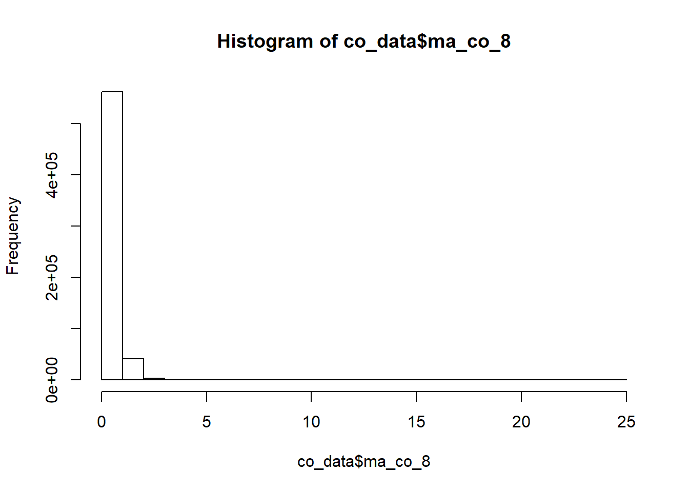

summary(co_data$ma_co_8)

##    Min. 1st Qu.  Median    Mean 3rd Qu.    Max.    NA's 
##    0.00    0.25    0.39    0.48    0.60   24.34  116415

plot(co_data$ma_co_8)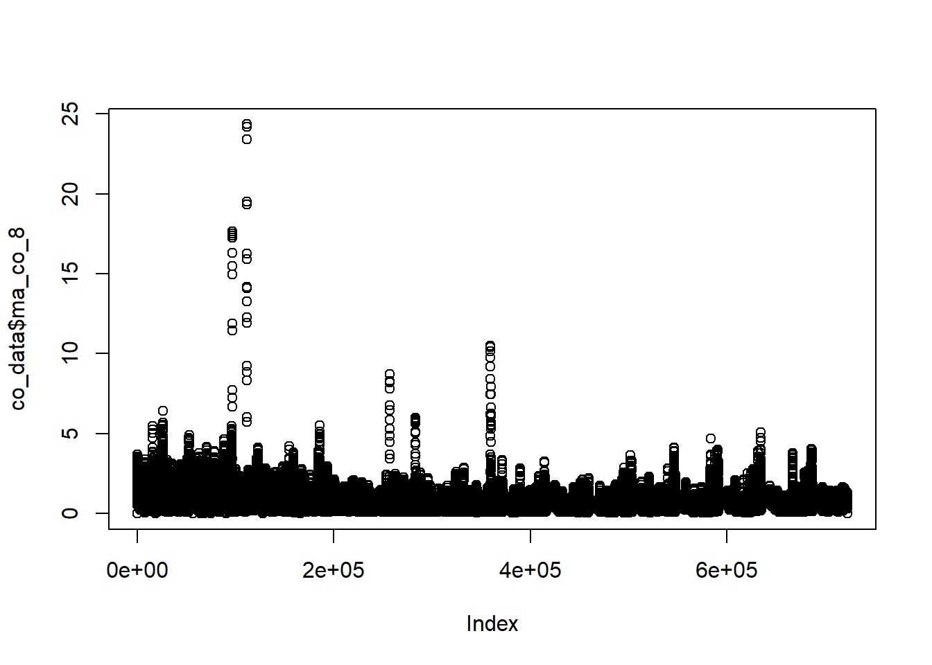

# pending na treatment

saveRDS(co_data, file = "data_rds/co_data.rds")
write_csv(co_data, "data_final_csvs/co_data.csv")

6.3.4.2 O3 tables

We create a O3 dataset with O3 Moving averages (each 8 hours). It is needed to measure the accomplishment of UE limits for this pollutant

o3_data <- air_data_2 %>% select(station_alias, date_time_utc, O3) %>%
                          mutate(ma_o3_8 = roll_mean(O3, 8, fill=0),
                                 o3_8_acc = ifelse(ma_o3_8 > 125, 'no', 'yes'))


hist(o3_data$ma_o3_8)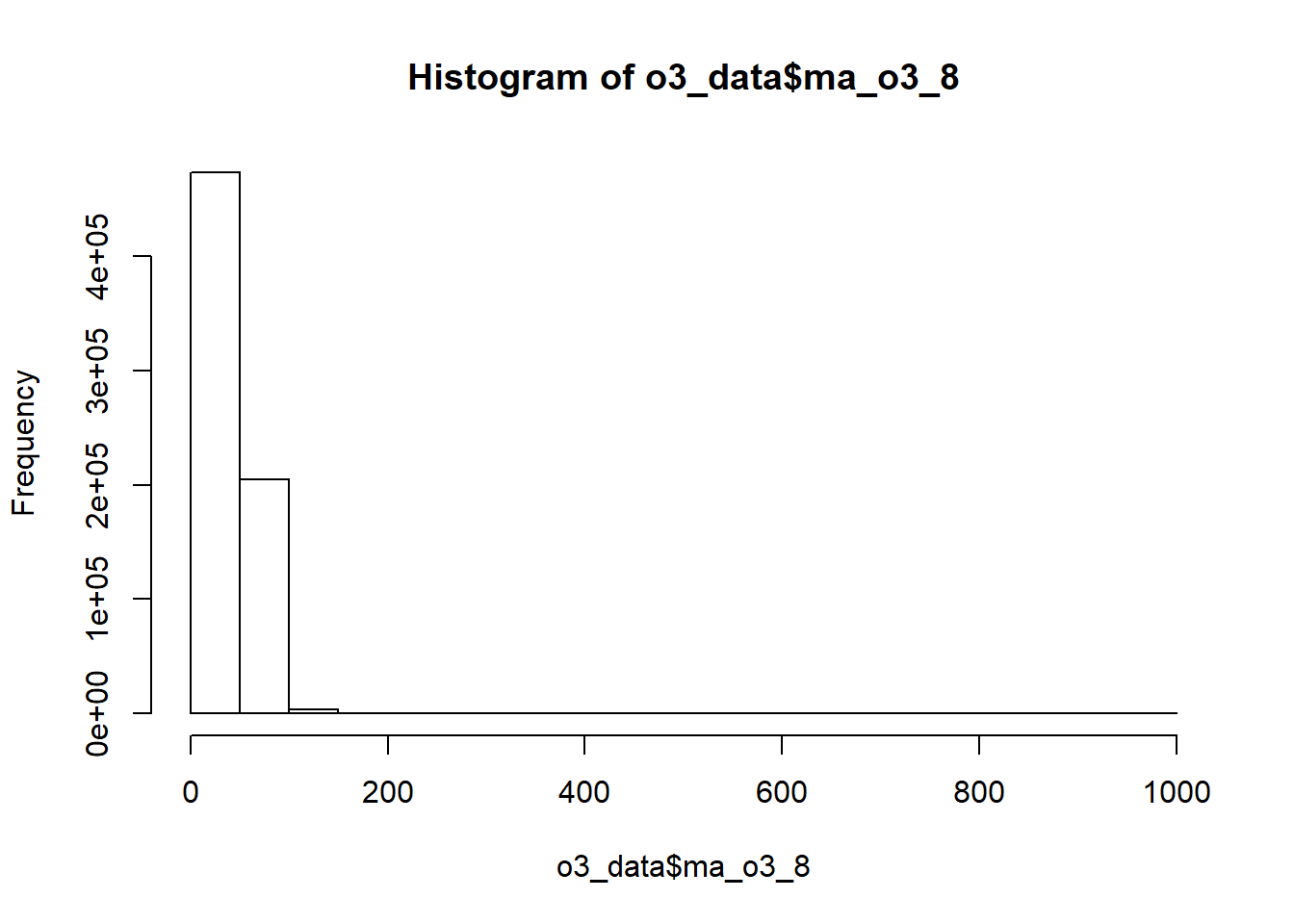

summary(o3_data$ma_o3_8)

##    Min. 1st Qu.  Median    Mean 3rd Qu.    Max.    NA's 
##    0.00   21.50   37.50   39.34   54.10  998.00   41435

plot(o3_data$ma_o3_8)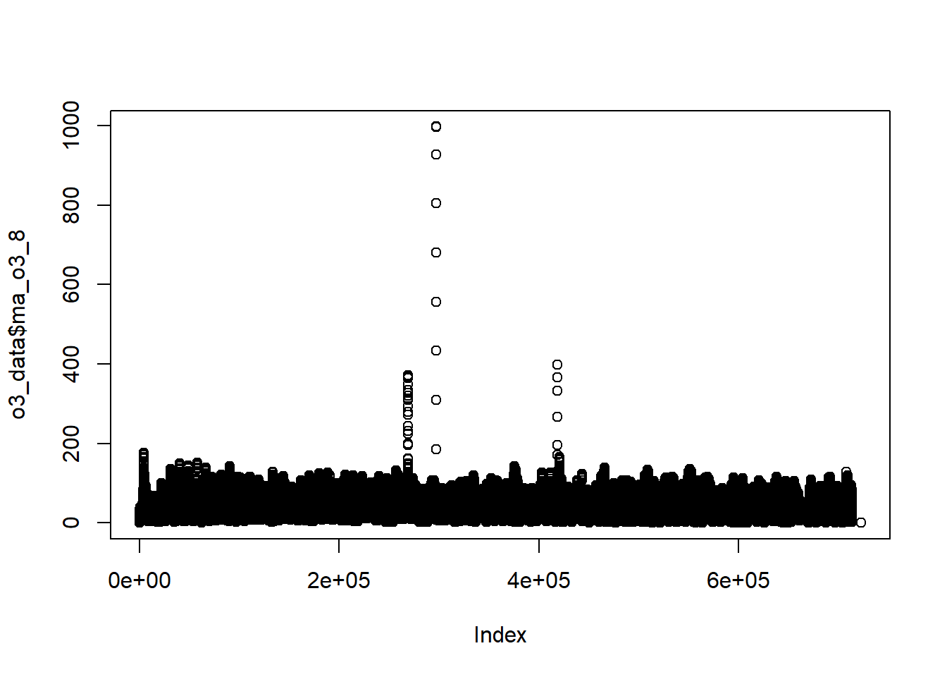

# pending na treatment

saveRDS(o3_data, file = "data_rds/o3_data.rds")
write_csv(o3_data, "data_final_csvs/o3_data.csv")

6.3.4.3 SO2 tables

RD 102/2011 Hourly limit: 350 ug/m3 (1 hour). <= 24 times / year. Daily limit: 125 ug/m3 (24 hours). <= 3 times / year. Alert threshold: 500 ug/m3 (3 hours).

so2_data <- air_data_2 %>% select(station_alias, date_time_utc, SO2)

saveRDS(so2_data, file = "data_rds/so2_data.rds")
write_csv(so2_data, "data_final_csvs/so2_data.csv")

# How many times was the Hourly limit exceeded during the last 18 years?

so2_hourly_limit <- so2_data %>%
                    group_by(station_alias,
                             year = year(date_time_utc),
                             day = date(date_time_utc)) %>%
                    filter(SO2 > 350) %>%
                    summarise(n = n()) %>%
                    arrange(year)


so2_hourly_limit

## # A tibble: 14 x 4
## # Groups:   station_alias, year [9]
##    station_alias  year day            n
##    <fct>         <dbl> <date>     <int>
##  1 Castilla       2001 2001-10-20     2
##  2 H. Felgueroso  2001 2001-10-20     2
##  3 Argentina      2004 2004-01-27     2
##  4 Argentina      2004 2004-01-28    12
##  5 Constitucion   2007 2007-05-30     1
##  6 Argentina      2008 2008-09-25     1
##  7 Argentina      2008 2008-11-27     1
##  8 Castilla       2008 2008-11-17     1
##  9 Castilla       2008 2008-12-25     4
## 10 Castilla       2008 2008-12-26     7
## 11 Castilla       2009 2009-01-05     1
## 12 Castilla       2011 2011-06-07     6
## 13 Castilla       2011 2011-06-08     1
## 14 Constitucion   2011 2011-01-13     3

saveRDS(so2_hourly_limit, file = "data_rds/so2_hourly_limit.rds")
write_csv(so2_hourly_limit, "data_final_csvs/so2_hourly_limit.csv")


# How many times was the Daily limit exceeded during the last 18 years?

so2_daily_limit <- so2_data %>%
                    group_by(station_alias, date = date(date_time_utc), year = year(date_time_utc)) %>%
                    summarise(avg = mean(SO2, na.rm = TRUE)) %>%
                    ungroup %>%
                    filter(avg > 125) %>%
                    group_by(station_alias, year, date) %>%
                    summarise(n = n()) %>%
                    arrange(year)



so2_daily_limit

## # A tibble: 6 x 4
## # Groups:   station_alias, year [3]
##   station_alias  year date           n
##   <fct>         <dbl> <date>     <int>
## 1 Argentina      2004 2004-01-28     1
## 2 Castilla       2008 2008-11-17     1
## 3 Castilla       2008 2008-12-25     1
## 4 Castilla       2008 2008-12-26     1
## 5 Castilla       2011 2011-06-07     1
## 6 Castilla       2011 2011-06-08     1

saveRDS(so2_daily_limit, file = "data_rds/so2_daily_limit.rds")
write_csv(so2_daily_limit, "data_final_csvs/so2_daily_limit.csv")