Chapter 3 Forest Erosion Control
The availability of sediment in torrent catchments is related to magnitude and frequency of torrential events. Within the scope of this chapter, the influence of forests on erosion and thus on the displacement of sediments is explained.
Torrential catchments are, beside being a drainage areas for precipitation, also sediment source zones of river systems. Steep headwater areas deliver significant volumes of sediment to the valley floor in highly dissected and coupled landscapes (Fryirs and Brierley 2013). Torrential catchments can thus be considered as temporally variable reservoirs of sediment that can be partially or fully incorporated into the flowing mass when they coincide with a critical precipitation event. Torrential processes such as sediment transport processes (Fig. 3.1), debris floods (Fig. 3.2) or debris flows (Fig. 3.3) are capable to relocate a considerable quantity of sediment in steep headwater torrents, often with tragic consequences on human settlements and infrastructures.

Figure 3.1: Typical section of a torrent with evidence of sediment transport processes.
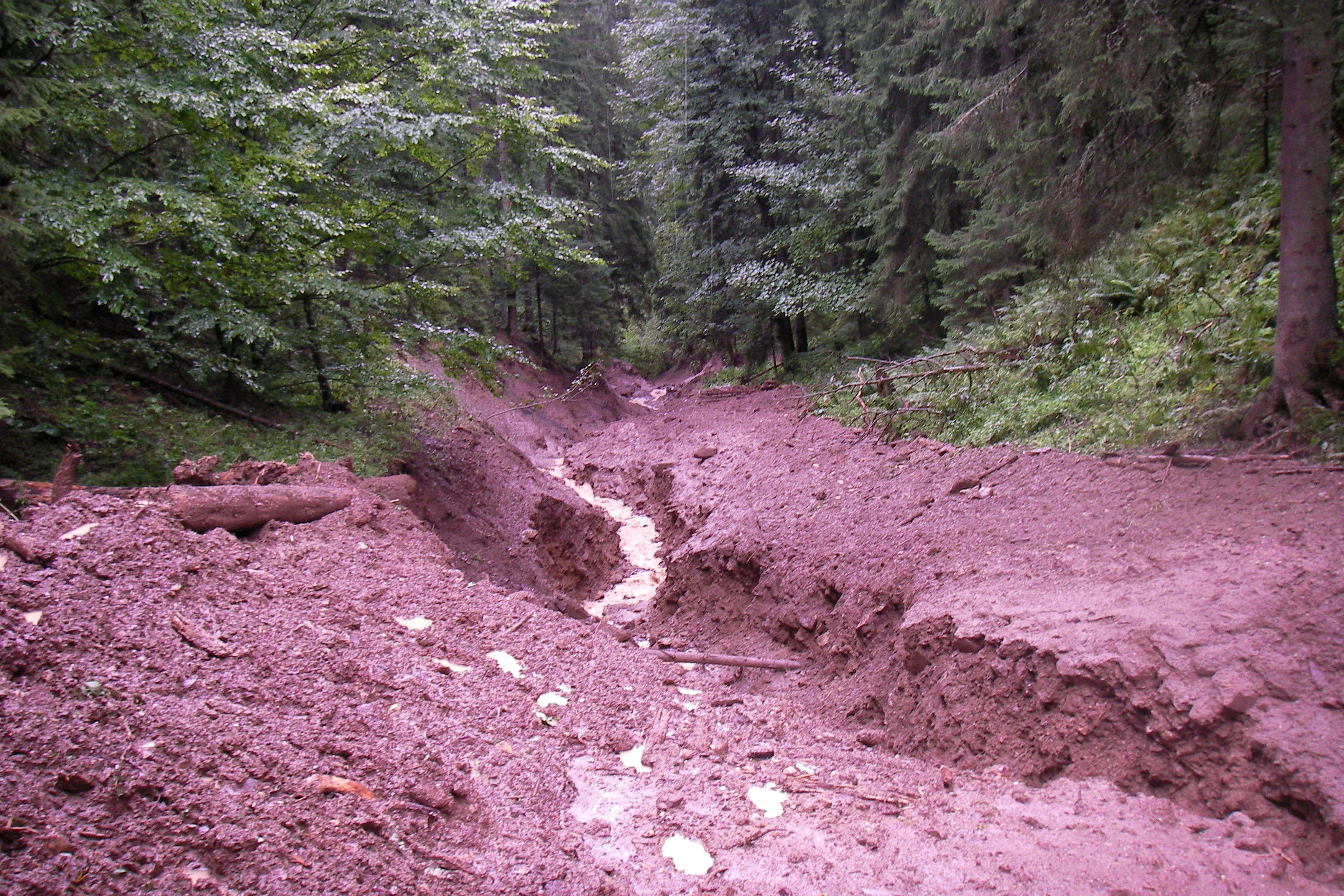
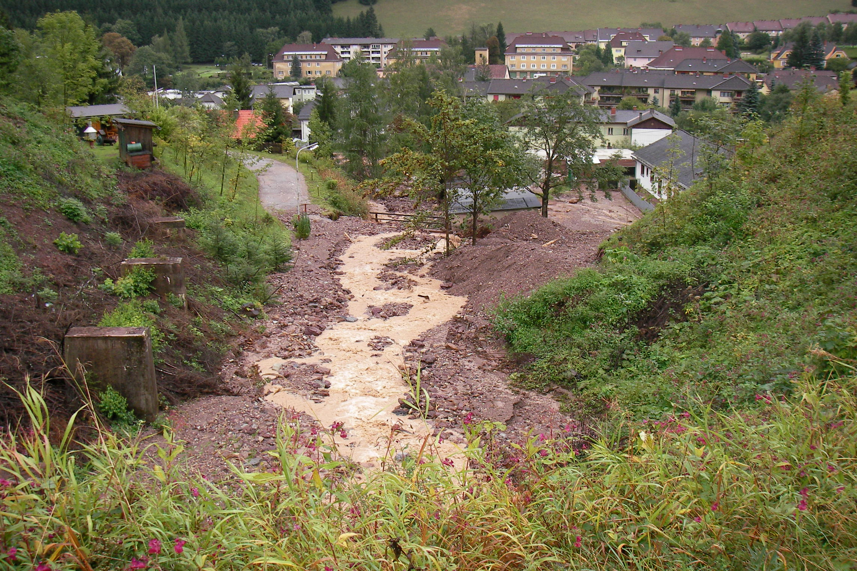
Figure 3.2: Debris-flood event, 2007 Tullbach (AUT)
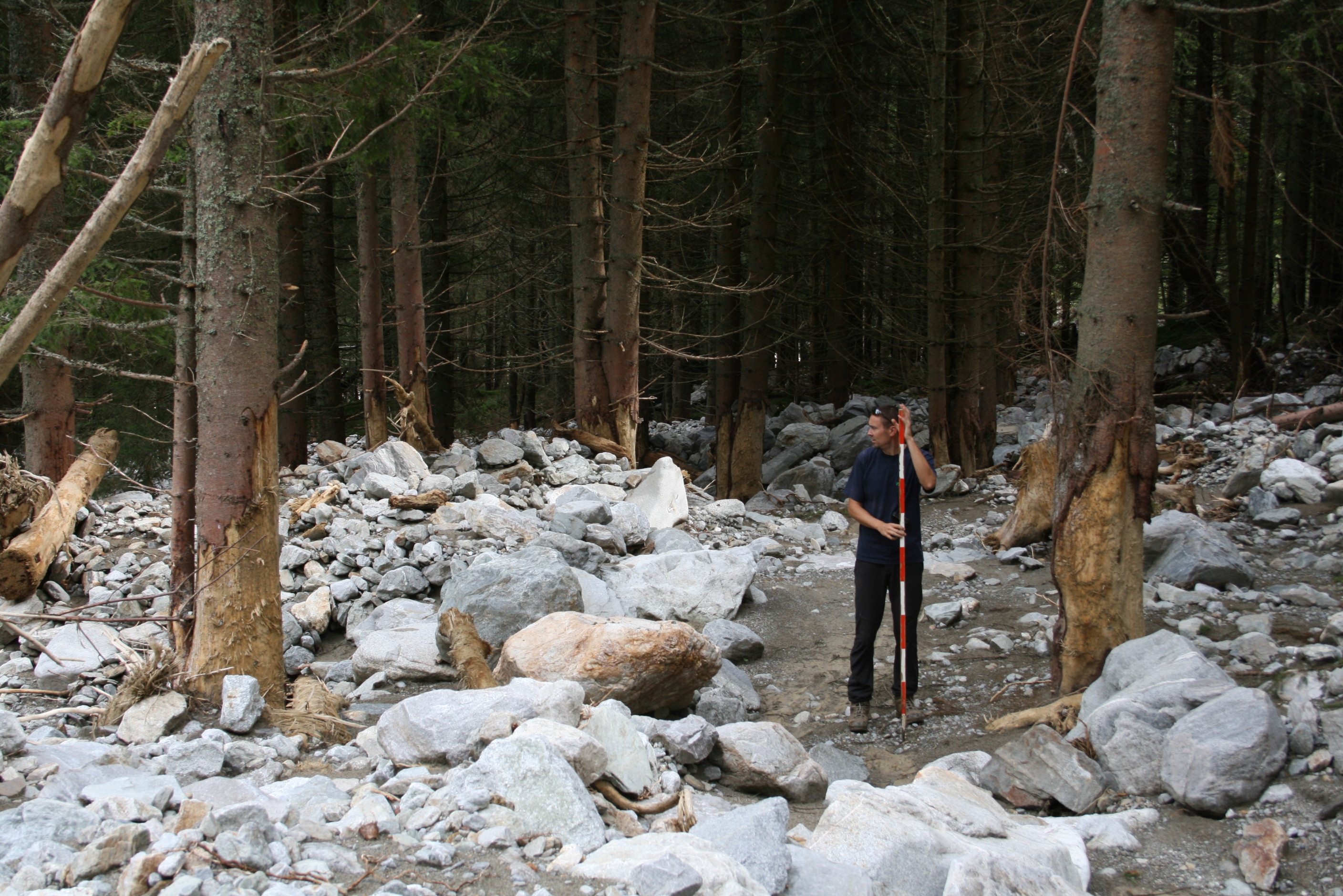
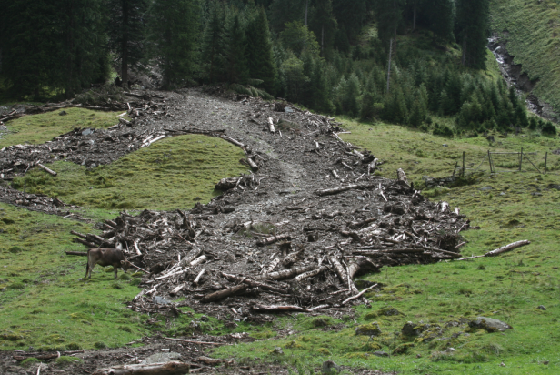
Figure 3.3: Debris-flow event, 2010; Sölktal (AUT)
Hence, the presence (or absence) and storage of sediment significantly controls the probability of occurrence and magnitude of torrential events. This means that the likelihood of torrential events to occur is a function of the availability of erodible sediments (within the whole catchment area), the occurrence probability of hill-slope failures, and the frequency at which certain intrinsic (location-based) or extrinsic (climatic) thresholds are exceeded (Jakob, Bovis, and Oden 2005). Bovis and Jakob (1999) established a differentiation between transport-limited basins in which an almost unlimited amount of sediment is available to feed torrential processes (supply-unlimited) and weathering-limited basins in which sediment supply and channel recharge rates are lower, and a substantial time period must elapse before the next torrential event is possible (supply-limited). They further proposed a constant threshold over time for supply-limited and transport-limited watersheds with respect to debris-flow initiation and report nearly 7 times higher debris flow activities in transport-limited basins (~8,000 \(m^3a^{-1}\)). With regard to sediment availability, the protective effect of a forest relates more to the erosion capacity within the catchment under consideration and thus to the sediment input from slope processes into the channel. Forest stands can interact between hillslope erosion processes (e.g. landslides) and the channel system - and as such indirectly influence the extent and frequency of torrential events.
With gravity as the main driving force, landslides occur when this driving force becomes greater than the resisting forces – triggered mainly by heavy rainfall and storm events, but also by earthquakes, volcanic activity or man-made building activities (forest streets) and forest clearing. The susceptibility of landslides is thus strongly related to topography and pedology (K. M. Schmidt et al. 2001) and researchers often attribute the seemingly stochastic occurrence of landslides to the spatial variations of topography, soil depth, cohesion from the soil and roots, hydraulic conductivity, groundwater response, and angle of internal friction (K. M. Schmidt et al. 2001; Dietrich et al. 2007). For this reason, recent erosion models, considering the effect of (forest) vegetation on slope stability, include a modification of soil moisture regime through evapotranspiration processes and the influence of root cohesion to the soil mantle (Anagnostopoulos, Fatichi, and Burlando 2015; Burton and Bathurst 1998; Cuo et al. 2008; Scheidl et al. 2020).
Generally, forests offer large scale protection considering landslide hazard prevention and mitigation. This is particularly important, since in contrast to other hazard processes, areas prone to landslide can be rarely identified prior to the event, limiting the use of technical protection measures (Scheidl et al. 2021). However, subsequent to catastrophic landslide events there is often controversy on forest management practices (K. M. Schmidt et al. 2001), since the magnitude of such effects can largely vary by forest type. Keppeler and Brown (1998) and Rickli (2001) report a close connection between forest condition and hillslope activity, while forest vegetation is known to increase hillslope stability mainly by reinforcing soil shear resistance and by influencing hydrologic conditions of soil (Bischetti et al. 2005). However, once mobilized, the influence of the forest on the respective transport rate of sediment is very low to nonexistent. On the contrary, in case of strong torrential floods, large wood recruitment is rather considered as an additional source of danger, which can lead to clogging and thus to stream displacements.
3.1 Root reinforcement
It is generally accepted that the root system of trees increases the resistance against shallow landslides by additively increasing soil cohesion through root reinforcement. Thus, if we consider the influence of the roots in terms of slope stability, it is described by the apparent cohesion that increases the resistant shear strength of the sliding mass under consideration. As evidenced in numerous studies, the effect of apparent cohesion (hereafter referred to as root cohesion \(c_r\)) has a significant effect on slope stability and, considering the decay of roots after deforestation, is also invariant over time (Chok et al. 2015).
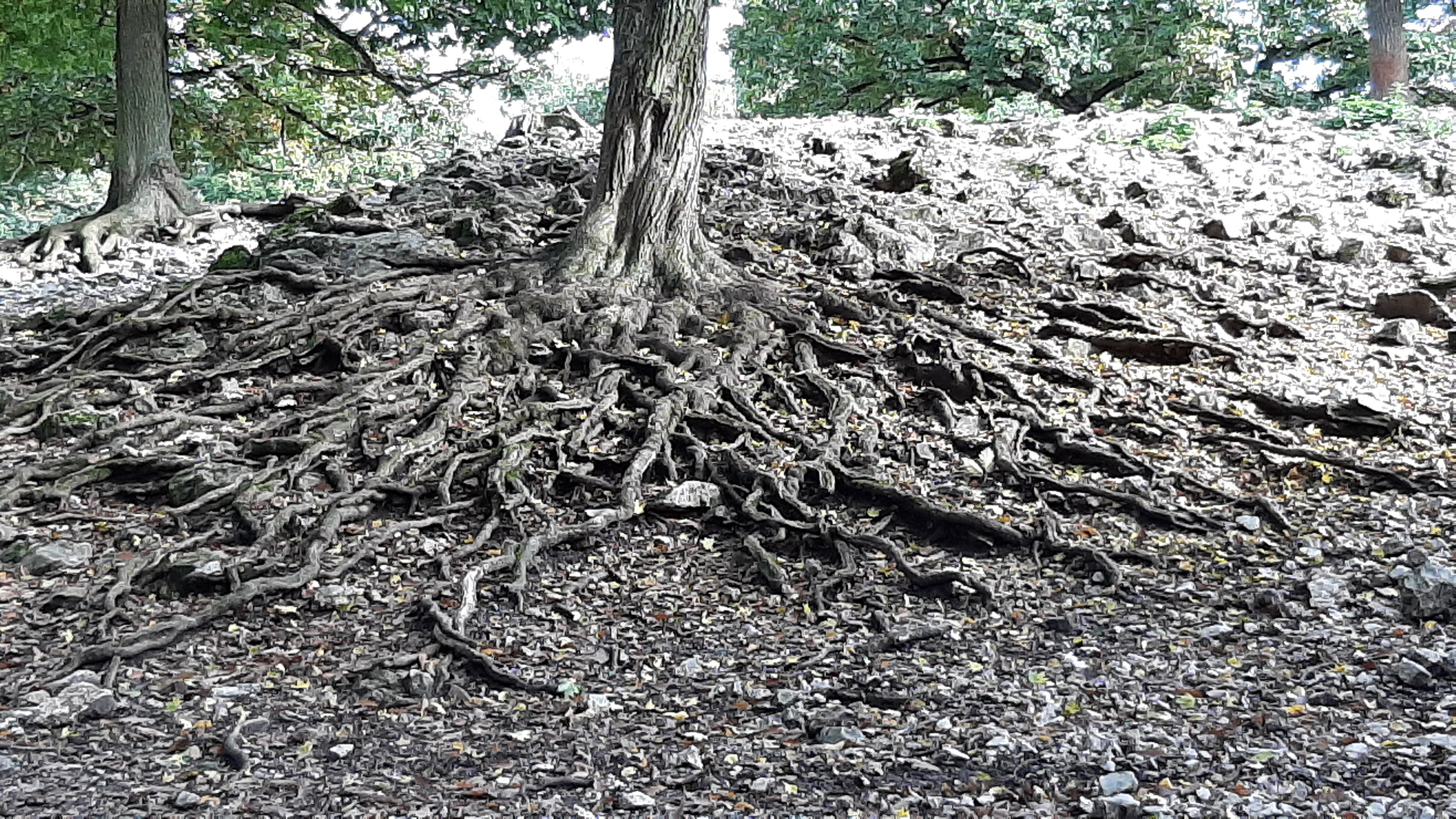
Figure 3.4: Root reinforcement acting as apparent cohesion of the upper soil layer.
Recent erosion models, considering the effect of (forest) vegetation on slope stability, often include therefore, beside a modification of soil moisture regime through evapotranspiration processes, the influence of root cohesion to the soil mantle (Anagnostopoulos, Fatichi, and Burlando 2015; Burton and Bathurst 1998; Cuo et al. 2008; Scheidl et al. 2020). However, root cohesion values for different tree species may vary over a wide range. The following table provide an overview of published root cohesion values of trees, estimated by in-situ field measurements.
| Root coehsion [kPa] | Tree species | Reference | ||
|---|---|---|---|---|
| Min. | Max. | Mean | ||
| 2.0 | 12.0 | - | Alder (Alnus japonica Steud.) in nursery | Endo and Tsuruta (1969) |
| - | - | 6.0 | Beech (Fagus sp.) | C. O’Loughlin and Ziemer (1982) |
| 3.0 | 21.0 | - | Lodgepole pine (Pinus contorta) | Ziemer (1981) |
| - | - | 3.3 | Radiata pine (Pinus radiate D. Don) | Colin O’Loughlin and Watson (1979) |
| 3.7 | 6.4 | - | Yellow pine (Pinus ponderosa) in laboratory | Waldron, Dakessian, and Nemson (1983) |
| 1.0 | 5,0 | - | Japanese cedar (Cryptomeria japonica) | Abe and Iwamoto (1986) |
| 0.6 | 18.2 | - | Aleppo pine (Pinus halepensis) | van Beek et al. (2005) |
Beside its variability with tree type, root cohesion also varies with age resulting in considerable spatial and temporal variations in the mosaic of stand density and tree composition. K. M. Schmidt et al. (2001) proposed root cohesion values to be uniformly less than 10 kPA in clear cuts, 6.8-23.2 kPA in industrial forests and 25.6-94.3 kPA in natural forests. The reason can be mainly attributed to the development and state of the root system, e.g. the vertical and lateral root distribution, which is a function of genetic properties of the species and site characteristics (soil texture and structure, aeration, moisture, temperature and competition with other plants). As the wide range of values already suggests, root cohesion is exceedingly difficult to measure and few studies have attempted to measure their spatial variation intrinsically at the scale that influences slope stability. It is difficult, however, to quantify soil–root pull-out resistance over large areas because of the branching, lateral network of roots, presence of root hairs, and interlocking nature of roots from separate plants. Thus, models of different degree of complexity to estimate root cohesion values have been proposed. Scheidl et al. (2020) defined the necessary root cohesion by quantile matching of modelled root mass distributions with literature-based log-normal root cohesion distributions for each tree species respectively root system.
3.1.1 The Wu-Model
A very commonly used approach is the simple perpendicular root model of Wu, McKinnell III, and Swanston (1979). Here, the magnitude of root cohesion (\(c_r\)) simply depends on the amount of roots present in the soil (\(RAR\)), a factor for root orientation (\(K\) [1.0-1.3]) and the strength of those roots (\(t_r\)).
\[\begin{equation} c_r=RAR\cdot K\cdot t_r \tag{3.1} \end{equation}\] with \[\begin{equation} RAR=\frac{A_r}{A}= \frac{\sum_{i=1}^{n} \pi {\Phi_i}^2}{4A} \tag{3.2} \end{equation}\]
The root-area-ratio (\(RAR\)) accounts for root distribution and is a function of \(A_r\) and \(A\), representing the cross-sectional area of root and soil, respectively; \(\Phi_i\) denotes the diameter of the \(i\) th root; and \(n\) is the total number of identified roots (cf. Feng, Liu, and Ng 2020). Although the Wu-model has a wide range of applications, it comes with some limitations and assumptions. First, the model assumes that roots are normal to the slip surface. This is not the case, especially on steeper slopes, because the angle of the roots with respect to the direction of the forces acting on the ground influences the maximum root tensile strength reached (lateral root reinforcement). Secondly, tortuosity is not considered, i.e. a pulling apart of the roots before there is a load that can be transferred to the soil. Third, the model does not account for the failure mechanism of pullout (slipping due to bond failure). A major problem for the implementation of the Wu-model is further the estimation of the root distribution, given as root-area-ratio (\(RAR\)). \(RAR\) provides a measure of root density within the soil and as a consequence it is strongly influenced by local soil and climate characteristics, land use management, and associated vegetation communities and randomness. In-situ measurements, e.g. counting roots within a known cross section area, can either be conducted by core-break sampling or profile trenching. Both methods are time-consuming, which is why they are usually only carried out for a representative site or tree species. However, this often leads to insufficient results since the root distribution is known to decrease with depth from the soil surface and distance from the trunk.
3.1.2 The Fiber-Bundle-Model
The fundamental weakness of the Wu-Model can be attributed to the fact that when a load is applied to the bundle of “root fibers”, they all break simultaneously. In fact, root reinforcement (peak) and soil peak strength take place at different time. To account for a progressive failure of soil–root systems, models for mechanical interactions of bundles of roots have been formulated within the formalism of the fiber bundle model (FBM) (Kun et al. 2006; Pollen and Simon 2005; Sornette 1989). Here, root reinforcement is calculated as a force (newtons) instead of a stress kPa and is the sum of the forces activated by each root. Only when we reference this force (e.g., at peak stage) to a surface area (e.g. a square meter in a vertical cross section) can root reinforcement be expressed as a stress in kPa (Giadrossich et al. 2016). Based on the FBM approach, Schwarz, Lehmann, and Or (2010) provided a modelling framework in steep slopes, which allows to consider the spatial distribution of root distribution (especially the lateral effect of roots) with explicit consideration of the structure of vegetation cover.
The root distribution model (RDM) proposed by Schwarz, Lehmann, and Or (2010) and applied in several studies (Schwarz, Cohen, and Or 2012; Giadrossich et al. 2019; Cislaghi et al. 2021) estimates in principle densities of roots for different size classes of individual stems for a 1 m wide and 1 m deep vertical section of soil (c.f. \(RAR\) in equation 2). The model combines a static fractal branching model and the pipe theory model Shinozaki et al. (1964). The RDM first estimates the density of fine roots \(FR\) (< 1.5 mm in diameter) at a given distance \(d\) from the tree stem based on the following relation (c.f. Vergani et al. 2017): \[\begin{equation} FR(DBH,d)=\left(\frac{\mu P}{d_{max}^{2\pi d}}\right)\left(\frac{d_{max}-d}{d_{max}}\right) \tag{3.3} \end{equation}\] With the maximum distance \(d_{max}\) commonly estimated by a linear function of the tree diameter in breast height (\(DBH\)). The principal number of roots per meter distance from the stem is given by \(\mu\), a coefficient based on pipe-theory reflecting allometric parameters (\(P\)) of a tree such as leaf area index, sapwood area, crown volume or stem diameter (Schwarz, Lehmann, and Or 2010). Vergani et al. (2017) referred for instance \(P\) in equation (3) to \({DBH}^2\frac{\pi}{4}\). The density of all roots at a distance \(d\), as a function of root diameter (\(\Phi_i\)) for diameter values between fine root size and coarse roots (> 1.5 mm in diameter), can then be calculated with: \[\begin{equation} R(d,\Phi_i)=FR(DBH,d)\left(\frac{ln(1+\Phi_{max}1000)-ln(1+\Phi_i)}{ln(1+\Phi_{max})}\right){\left(\frac{\Phi_i}{\Phi_0}\right)}^\gamma \tag{3.4} \end{equation}\] where \(\gamma\) is a constant exponent (fractal branching), \(\Phi_i\) (mm) is the root diameter in the class \(i\), \(\Phi_0\) is a reference diameter (1 mm), and \(\Phi_{max}\) (mm) is the diameter of the largest root at a distance \(d\) from the stem. \(\Phi_{max}\) is given by: \[\begin{equation} \Phi_{max}=\frac{d_{max}-d}{\eta} \tag{3.5} \end{equation}\] With \(\eta\) a dimensionless scaling coefficient that describes the fractal root branching by assuming a constant value for the branching distance at which a coarse root can split into roots with finer diameter in a constant proportional way. The concept of the RDM enables a direct parameterization independently of in-situ measurements due to allometric relationships between trees and the root system by applying pipe model theory (Shinozaki et al. 1964). This theory views the stem as a series of pipes, that link roots with foliage. The theory states that trees maintain a constant amount of leaf dry matter per unit of cross-sectional area of active pipes throughout the crown. As outlined above, the concept allows to calculate the spatial distribution of rooting distribution at the stand level. Empirical knowledge of the spatial distribution of root frequencies and sizes is, however key to quantify the root reinforcement.
The Root Bundle Model Weibull (RBMw), proposed by Schwarz, Giadrossich, and Cohen (2013), can be considered as the state of the art for quantifying root reinforcement. The RBMw estimates the total force of a root bundle (\(F_{tot}\)) by summing up individual root forces as a function of average root-diameter per class (\(\langle\varphi_i\rangle\)) and displacement (\(x\)), and whose failure is given by a Weibull-distributed survival function (\(S\)) depending on normalized displacement (\(\xi_i\)). \[\begin{equation} F_{tot}(x)=\sum\limits_{i=1}^{N}[(n_iF(\langle\varphi_i\rangle,x)S(\xi_i)] \tag{3.6} \end{equation}\] Here, \(N\) corresponds to the maximum root diameter class and \(n_i\) is the number of roots within class \(i\) as estimated by the RDM. Individual root forces (\(F(\langle\varphi_i \rangle,x)\)) as well as normalized displacement (\(\xi_i\)) have to be known or calibrated, based on in-situ tensile strength tests. For a test site located at the Rhine valley (350 m a.s.l.) with a mull humus layer (Schwarz, Cohen, and Or 2012) used a pipe coefficient of \(\mu=0.09\) and the lateral rooting extend was \(d_{max}=2 m\) for a \(10\) cm tree, and \(d_{max}=6.5 m\) for a \(50\) cm tree (Schwarz, Cohen, and Or 2012). He could then show for individual trees that maximum root reinforcement decreases with the distance from the tree (Schwarz, Cohen, and Or 2012) and is considerably smaller for young trees. At the stand level, this may however be outweight by the higher number of small trees in the stand. Such stand level simulations of the root reinforcement of homogeneously and regularly distributed forest stands were presented and gave valuable insights, even though some of the assumptions made on the forest are highly unrealistic. For example, stand basal areas used in these simulations were 40, 120, and 230 \(m^2 ha^{−1}\) and the latter two basal areas are considerably higher than maximum basal areas or 40-80 \(m^2 ha^{−1}\) observed by the Austrian National Forest Inventory for different tree species (Vospernik and Sterba 2015).
However, differences between measured and modelled root distribution values can lead to errors of \(28 \%\) (Schwarz, Cohen, and Or 2012) and it is therefore important to obtain precise empirical root measurements. As a kind of standard method for measuring the root distribution, trenches at three different distances from the tree under consideration have proven successful. Root parameters that need to be calibrated, by minimizing squares errors (i.e.: Root Mean Square Error, Mean Absolute Percentage Error) between predicted (RDM) and compiled root distribution, data are:
- \(\mu\), the pipe coefficient, considered in this project as a function of the LAI,
- \(\psi\), the proportionality coefficient as a function of the DBH,
- \(\eta\), the fractal root branching coefficient,
- \(\gamma\), root density decrease coefficient.
To predict the spatial distribution of root reinforcement, different approaches exist. Moos et al. (2016) and Dazio, Conedera, and Schwarz (2018) estimated the effect of root reinforcement on an areal stand level, which follows a gamma distribution, depending on BHD and distance from the tree trunk. Based on the Virtual Random Forest (VRF) model, Cislaghi et al. (2021) estimated the spatial distribution of root reinforcement for a set of virtual forests of randomly located trees. For Norway spruce in particular, they found very good agreement between the root reinforcements calibrated based on field surveys and those calibrated based on the virtual forest.