Chapter 6 TODO: affect speed based through transitions based on genetics
To estimate the speed through a topic for a given polygenic score in a large-scale simulation, and to predict at what age diseases might occur for an individual, you can integrate the concept of a polygenic score into your topic model. This requires a nuanced approach where the polygenic score influences the rate of progression through a topic. The idea is similar to genetic penetrance, where certain genetic factors might lead to earlier or later onset of diseases.
Steps to Integrate Polygenic Score: 1. Incorporate Polygenic Score in the Model:
Polygenic Score (PGS): Assume each individual has a polygenic score that quantifies their genetic predisposition towards certain diseases or disease progressions. Model Adjustment: Adjust the dynamics of your topic model based on the PGS. Higher scores might imply earlier onset or faster progression through disease stages within a topic. 2. Modifying Spline Dynamics Based on PGS:
Dynamic Splines: Use the PGS to alter the parameters of the spline functions governing the transition through topics. For example, individuals with a high PGS might have spline functions that shift the disease probabilities to earlier ages.
Time Scaling: Consider scaling the time axis based on PGS. For instance, you can modify the time points at which the spline is evaluated, effectively ‘compressing’ or ‘expanding’ the time scale for individuals with higher or lower PGS, respectively.
# Function to scale PRS from a normal distribution to a [0, 1] range
scale_prs <- function(prs) {
  # Normalize PRS to be between 0 and 1
  # This is a simple min-max scaling; you can also consider other scaling methods
  scaled_prs <- (prs - min(prs)) / (max(prs) - min(prs))
  return(scaled_prs)
}

# Generate PRS for each individual - normally distributed

N_individuals <- 100  # Number of individuals
prs_raw <- rnorm(N_individuals, mean = 0, sd = 1)
prs_values <- scale_prs(prs_raw)

# Simulate PGS values for individuals

# Create an array to store individual-specific phi values, initialize with same for all
phi_base <- matrix(nrow = K, ncol = V)

for (k in 1:K) {
    beta <- rep(1/V, V)  # Start with low probabilities

    # Set higher probabilities for topic-specific diseases
    for (v in topic_spec_disease[k,]) {
        beta[v] <- (V-d)/V
    }

    # Initialize baseline phi for topic k using a Dirichlet distribution
    phi_base[k, ] <- rdirichlet(1, beta)
}

## check to make sure mostly topic hits
which(order(phi_base[1,],decreasing = T)%in%topic_spec_disease[1,])
## [1] 1 2 3 4 5 7 8 9 10 11# Expand phi_base to create the initial phi array for all individuals
phi <- array(dim = c(length(prs_values), V, K, length(time_points)))
for (i in 1:length(prs_values)) {
phi[i, , , 1] <- t(phi_base) # Set the baseline phi for each individual
}
## check to make sure mostly topic hits
which(order(phi[i,,1,1],decreasing = T)%in%topic_spec_disease[1,])## [1] 1 2 3 4 5 7 8 9 10 11## [1] 1 2 4 5 6 8 10 12 13 14## Min. 1st Qu. Median Mean 3rd Qu. Max.
## 5 5 5 5 5 5all_normalized <- all(apply(phi[,, , 1], c(1,3), function(x) abs(sum(x) - 1) < .Machine$double.eps^0.5))
print(all_normalized) # Sh## [1] TRUE# Functions to calculate the effects of PRS on the spline coefficients and time scale
# can't change coefficient if constained to proper probability distirbution
time_scale_adjustment <- function(prs) {
# Define the relationship between PRS and time scale
# This is a placeholder; you need to define how PRS affects time scale
return(1 - prs) # PRS compresses time scale
}
# Apply time scale adjustment based on PRS
for (k in 1:K) {
for (v in 1:V) {
# Use base coefficients for the spline, should be same for every person, only the time scale changes
base_coef <- runif(length(knots) + degree + 1, min = 0, max = 5)
for (i in 1:length(prs_values)) {
# Adjust time points based on individual's PRS
prs_time <- time_scale_adjustment(prs_values[i])
adjusted_time_points <- time_points[-1] * prs_time
# Re-calculate the spline basis for the adjusted time points
adjusted_bspline_basis <-
bs(
adjusted_time_points,
knots = knots,
degree = degree,
intercept = TRUE
)
# Calculate spline values with base coefficients
spline_values <- adjusted_bspline_basis %*% base_coef
# Store the values in phi, normalized across diseases at each time point
phi[i, v , k ,-1] <- spline_values * phi[i, v, k, 1]
# Normalize the values across diseases
}
}
}
high=order(prs_values,decreasing = TRUE)[3]
low=order(prs_values,decreasing = FALSE)[3]
## check to make sure same at time 1
sapply(seq(1:K),function(k){all.equal(phi[high,,k,1],phi[low,,k,1])})## [1] TRUE TRUE TRUE TRUE TRUE## normalize to a proper distribution
for(i in 1:length(prs_values)){
for(k in 1:K){
for(t in 1:T){
phi[i,,k,t]/sum(phi[i,,k,t])
}}}
## check to make sure still same at time 1
sapply(seq(1:K),function(k){all.equal(phi[high,,k,1],phi[low,,k,1])})## [1] TRUE TRUE TRUE TRUE TRUEall_normalized <- all(apply(phi[,, , 1], c(1,3), function(x) abs(sum(x) - 1) < .Machine$double.eps^0.5))
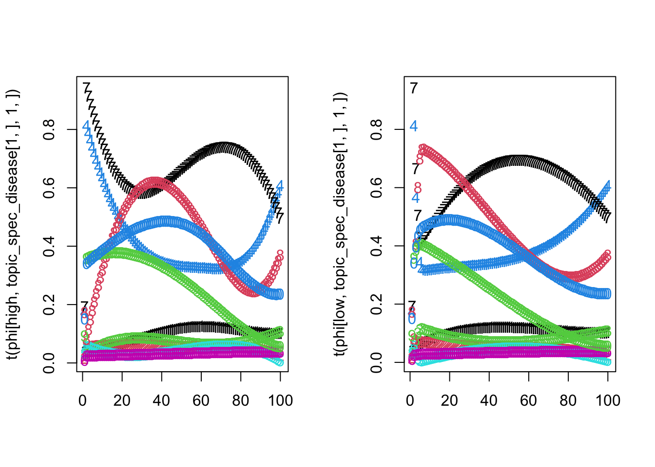
print(all_normalized) ## [1] TRUESo now we can visualize someone with a high risk and low risk PRS loaded on same topic:
high=order(prs_values,decreasing = TRUE)[3]
low=order(prs_values,decreasing = FALSE)[3]

## check to make sure initailization same
sapply(seq(1:K),function(k){all.equal(phi[high,,k,1],phi[low,,k,1])})
## [1] TRUE TRUE TRUE TRUE TRUEpar(mfrow=c(1,2))
matplot(t(phi[high,topic_spec_disease[1,],1,]))
matplot(t(phi[low,topic_spec_disease[1,],1,]))