Chapter 3 Simulation
Here we lay the grounds for a basic simulation.
For each patients, we simulate his \(N_{i}\) observed disease topic identities Z_{ij} according to his distribtuion of \(\theta_{i}\) We restrict so that the disease is assigned only once (in the setting of hesin choosing minimum age of diagnsoses)We explore how most of the observed diagnoses arose from one of the topic specific diseases (according to _{k})
library(rBeta2009)
library(ggplot2)
library(reshape2)
library(splines)

# number of people
M=100

# number of topics
K=5

## number of diagnoses per patient, mean of 10 diagnoses per patient
Nd=rpois(M,lambda = 10)

## total numer of diagnoses
N=sum(Nd)

# number of disease total
V=300
3.1 Simulate his \(N_{i}\) observed disease topic identities Z_{ij} according to his distribtuion of \(\theta_{i}\)
## make sparse so that most mass concentrated on one topic
alpha=rep(0.1,K)

#alpha=rep(1/K,K)

beta=rep(1/V,V)

## distribution of topics per pt
theta=rdirichlet(M,shape = alpha)
dim(theta)
## [1] 100 5## distribution of diseases per topic, load heavily on some
# d will be number of strong disease per topic
d=10
topic_spec_disease=matrix(sample(V,size = K*d),nrow=K,byrow = T)
phi=rdirichlet(K,shape = beta)
for (k in 1:K) {
for (v in 1:V) {
# Assign higher probabilities to certain diseases for each topic
# Placeholder: Assigning higher weights to some diseases
if (v%in%topic_spec_disease[k,]) {
beta[v] <- 1
} else {
beta[v] <- 1/V
}
}
phi[k, ] <- rdirichlet(1, beta)
}
dim(phi)## [1] 5 300# check to make sure topic specific disease highly loaded
which(order(phi[1,],decreasing = T)%in%topic_spec_disease[1,])## [1] 1 2 3 4 6 8 9 10 14 15## [1] 1 2 3 4 5 6 7 9 10 11## [1] 1 2 4 5 6 7 8 10 12 14## [1] 1 2 4 5 6 7 8 9 11 12## [1] 1 2 3 4 5 6 7 8 9 10disease <- list() # Initialize the list outside the loop
for (i in 1:M) {
# Check if the patient has any diagnoses to assign
if (Nd[i] > 0) {
disease[[i]] <- vector("list", Nd[i]) # Initialize the ith list if diagnoses are to be assigned
assigned_diagnoses <- integer(0) # Keep track of diagnoses already assigned to this patient
for (j in 1:Nd[i]) {
## for exah diagnosis, assign a topic
zij <- which(rmultinom(1, size = 1, prob = theta[i,]) == 1)
# Exclude already assigned diagnoses when selecting a new one
valid_diagnoses <- setdiff(1:V, assigned_diagnoses)
# normalize so sums to 1
prob_valid_diagnoses <- phi[zij, valid_diagnoses] / sum(phi[zij, valid_diagnoses])
if (length(valid_diagnoses) > 0) {
wij <- sample(valid_diagnoses, 1, prob = prob_valid_diagnoses)
disease[[i]][[j]] <- wij
assigned_diagnoses <- c(assigned_diagnoses, wij) # Update the list of assigned diagnoses
} else {
# Handle the case where all diagnoses have been assigned
# Placeholder: Assign a random diagnosis or handle as per your model's requirements
disease[[i]][[j]] <- sample(1:V, 1)
}
}
} else {
disease[[i]] <- NULL # Assign NULL or an appropriate placeholder for patients with no diagnoses
}
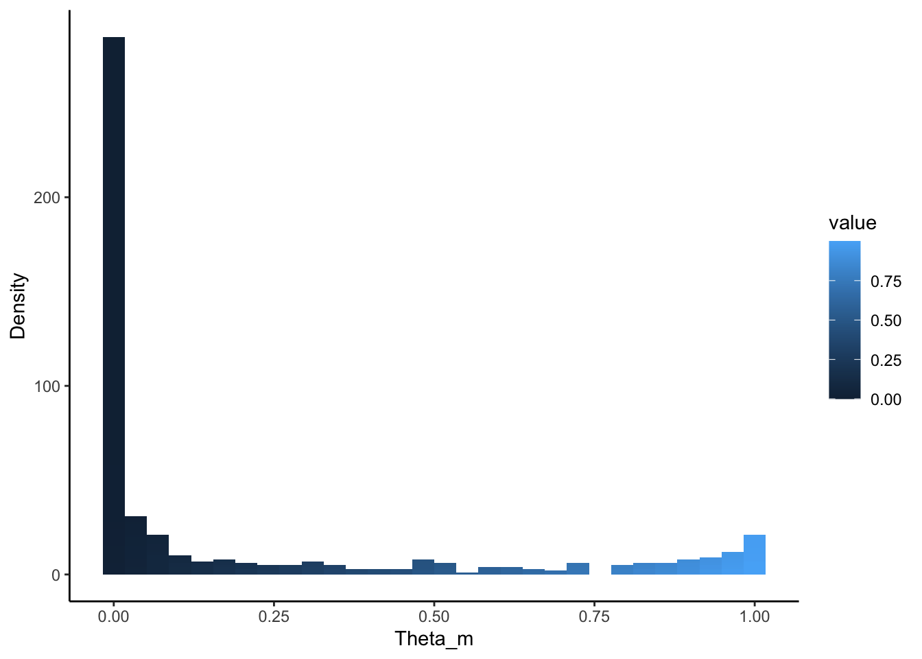
}3.2 Visualizing Basic Simulation
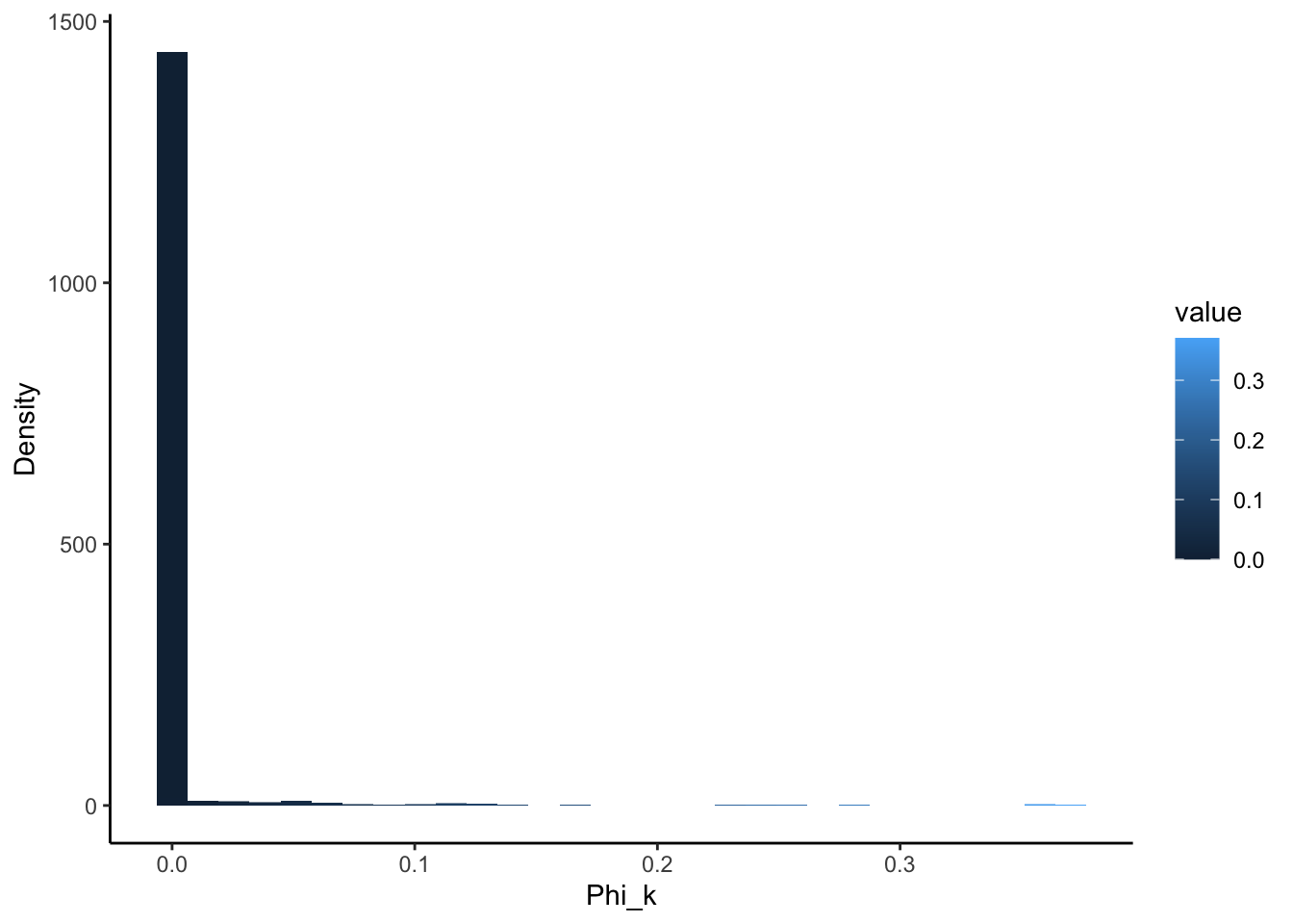
Here we whow the distirbtuion of \(theta\) and \(phi\) to demonstrate that individuals are minimally loaded on one topic and each topic is minimally loaded on a few diseases:
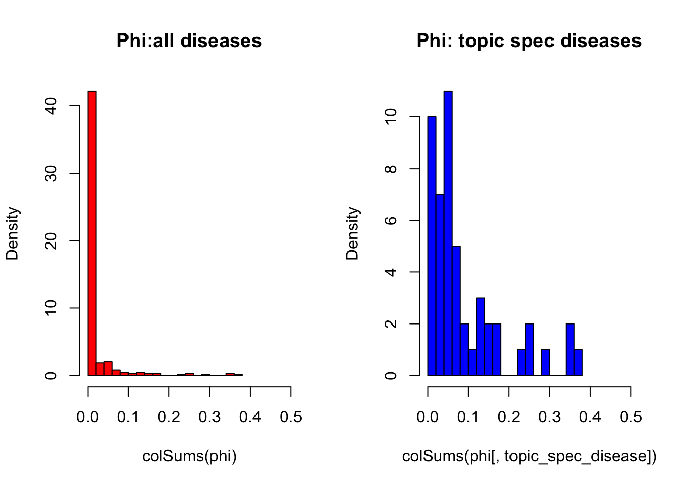
But overall, `we can see that topic specific diseases have a higher \(phi\) than those that don’t:
3.3 Observed data
Now, we want to observe the observed diagnoses \(w_{ij}\) for sample individuals
# Assuming 'disease' is your list of diagnoses for each person from above
# Convert 'disease' list into a data frame for plotting

disease_data <- data.frame(person = rep(seq_along(disease), sapply(disease, length)),
                        disease = unlist(disease))

# Now create the plot
random_peeps=sample(M,size = 5)
apply(theta[random_peeps,],1,which.max)
## [1] 3 1 2 4 1ggplot(disease_data[disease_data$person%in%random_peeps,], aes(x = disease,fill=as.factor(disease))) +
geom_bar() +
facet_wrap(~ person, scales = "free_x") +
theme(axis.text.x = element_text(angle = 45, hjust = 1)) +
labs(x = "Disease", y = "Frequency", title = "Disease Distribution per Person",fill="Disease")+theme_classic()
We can see that most people have on average 10 diagnoses from a set of V = 300. The people we choose, 47, 24, 5, 88, 86, were heavily loaded on the following topics:
3, 1, 2, 4, 1
For example, our first person 47 has 12 diagnoses. He is most heavily loaded on 3. In turn this topic was chosen to have concentration of \(phi_{k}\) at 169, 229, 254, 195, 125, 203, 9, 185, 191, 216 these disease.
We can see that a high proportion of his diagnoses emanate from one of these topic-specific diseases, which are
169, 254, 195, 229, 113, 9, 191, 247, 289, 153, 125, 177.
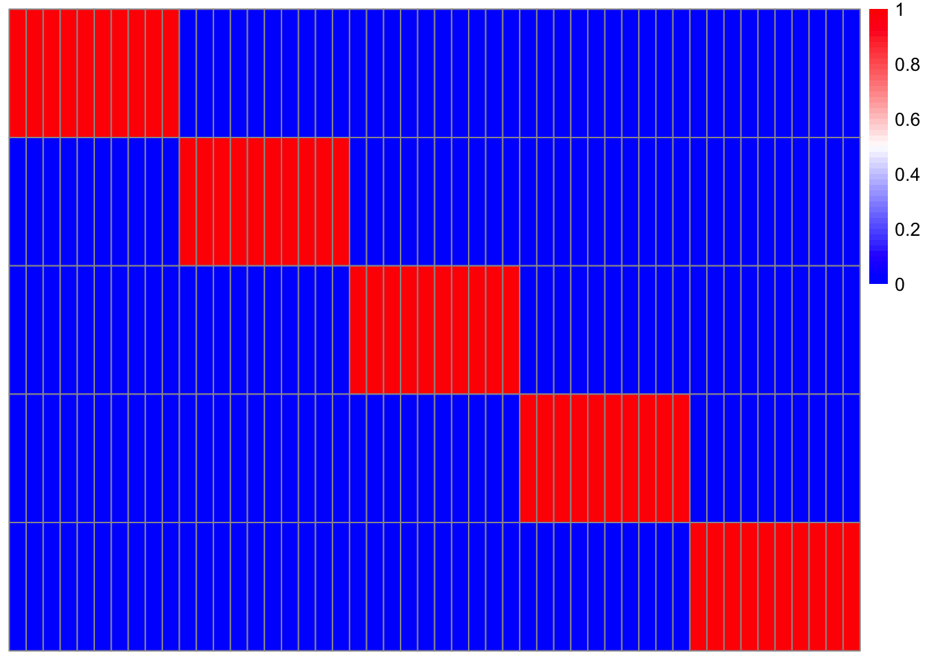
3.4 heatmap of people by disease
Now we plot a heatmap of disease diagnosis by patient (red is disease) and see how it reoughly paralelels the topic specific disease assignmetns.
library(tidyr)
library(dplyr)
library(pheatmap)

# Assuming 'disease_data' and 'topic_spec_disease' are your dataframes

# Create an empty matrix with 0s
expanded_patient_matrix <- matrix(0, nrow = 100, ncol = V)

# Fill in the matrix with 1s for diseases present in disease_data
for (row in 1:nrow(disease_data)) {
    expanded_patient_matrix[disease_data[row, "person"], disease_data[row, "disease"]] <- 1
}

topic_diseases <- as.vector(t(topic_spec_disease))
# Reorder the columns of expanded_patient_matrix
patient_matrix_reordered <- expanded_patient_matrix[, topic_diseases]

library(pheatmap)

# Generate the heatmap with row clustering
pheatmap(patient_matrix_reordered,
         color = colorRampPalette(c("blue", "white", "red"))(50),
         show_rownames = FALSE,
         show_colnames = TRUE,
         cluster_rows = TRUE,
         cluster_cols = FALSE,
         treeheight_row = 0,
treeheight_col = 0) 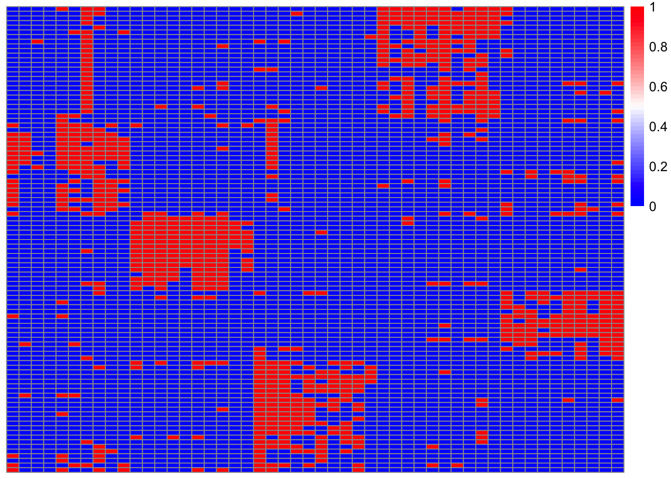
# For the topic data heatmap, disable clustering
binary_topic_matrix <- matrix(0, nrow = K, ncol = V)

# Fill the matrix with 1s based on topic-specific diseases
binary_topic_matrix <- matrix(0, nrow = nrow(topic_spec_disease), ncol = V)  # V is the total number of diseases

# Fill the matrix with 1s based on topic-specific diseases
for (i in 1:nrow(topic_spec_disease)) {
    binary_topic_matrix[i, topic_spec_disease[i,]] <- 1
}

binary_topic_matrix_reordered <- binary_topic_matrix[, topic_diseases]

pheatmap(binary_topic_matrix_reordered,
         color = colorRampPalette(c("blue", "white", "red"))(50),
         show_rownames = TRUE,
         show_colnames = TRUE,
         cluster_rows = FALSE,
         cluster_cols = FALSE, treeheight_row = 0,  # Set dendrogram height to 0 for rows
         treeheight_col = 0)