Chapter 5 However this assumes that an individual stays within a topic
Assumption: that the change in disease distribtuion for a given topic captures all the heterogeneity of disease coding
We know that is not the case from our previous work: an individual can switch to a new pattern based on genetics and environmental factors, and we should have an ability to ‘update’ an individuals’ topic distribtuion
Furthermore, genetics has a declining importance over time, and the new diagnoses carry more weight. The rate of advancement through a topic (i.e., the shape of the spline) also may be affected by these intrinsic factors
Finally, occupancy in one topic necessarily may prevent other topics
5.1 Example function to update theta based on new diagnosis
Let’s start by modeling an individual’s transition to a new topic distribtuion as a funciton of genetics.
That is, \(p(K=k|D)=p(D|K)*p(K)/p(D)\)
Here, we will have the genetics influence change by a decay factor, and the updated theta be proportional to the likelihood of the new diagnosis:
\(\theta_{t+1}=p(D|\theta_{t})*p(\tilde{\theta})\)
Here, \(p(\tilde{\theta}\) represents the genetics-adapted prior distribution
Genetics keeps us in the prior distribtuion more at early ages than later, so the strength of genetics influence on the prior will decline over time
library(rBeta2009)
update_theta <- function(current_theta, new_diagnosis, phi_time_dependent, genetics_influence, current_time, max_time) {
  # Ensure valid inputs
  if (any(is.na(current_theta)) || any(is.na(phi_time_dependent))) {
    #print("isna")
    return(current_theta)
  }

  # Decay factor for genetics influence
  decay_factor <- ((max_time - current_time) / max_time)^3


  adjusted_genetics_influence <- genetics_influence * decay_factor
  #print(adjusted_genetics_influence)

  # Select phi for the current time
  phi_current_time <- phi_time_dependent[,,current_time]

  # Adjusted prior as a vector, where genetics impacts less with tim
  adjusted_prior <- current_theta * adjusted_genetics_influence

  # Likelihood as a vector for the specific diagnosis
  likelihood_vector <- phi_current_time[, new_diagnosis]

  # Bayesian update: Element-wise multiplication of adjusted_prior and likelihood_vector
  updated_theta <- adjusted_prior * likelihood_vector

  # Check for zero likelihood and revert to original theta for those cases
  if (all(likelihood_vector == 0)) {
    return(current_theta)
  }

  # Normalize the updated theta
  total <- sum(updated_theta)
  if (total == 0 || is.na(total)) {
    return(current_theta)
  }

  return(updated_theta / total)
}
Simulate data, this time let’s let the topic distribtuion for an individual be roughly uniform on the simplex. Recall that if all are equal and greater than 1 (e.g., 100 for topic-specific diseases and 100 for non-topic-specific diseases), the distribution is centered around the vector (1/K, 1/K, …, 1/K). The higher the α values, the more peaked or concentrated the distribution is around this central vector.
M <- 400          # Number of patients
K <- 5            # Number of topics
V <- 300          # Number of diseases
T <- 100          # Number of time steps
max_time <- T     # Assuming T is the maximum time

# Initial topic distributions (theta) for each patient, we want this initially quite monotone at 1/K
initial_theta <- rdirichlet(M, shape = rep(100, K))


# Time-varying disease distributions within topics (phi)
# Assuming phi is a 3D array (topics x diseases x time)
# This needs to be defined based on your model

# Genetics influence (for simplicity, assuming a constant vector for each patient), how much they want to stay in a topic, but since we simulate topics randomly maybe think a bit more carefully about this
genetics_influence <- matrix(runif(M * K, 0.5, 1.5), nrow = M, ncol = K)

# Structure to hold theta values over time for each patient
theta_over_time <- array(dim = c(T, M, K))
theta_over_time[1, , ] <- initial_theta

## check to make sure all 1
all.equal(rowSums(theta_over_time[1,,]),rep(1,nrow(theta_over_time[1,,])))
## [1] TRUE# Function to simulate a new diagnosis (placeholder)
simulate_new_diagnosis <- function() {
# Randomly simulate a new diagnosis
return(sample(as.vector(topic_spec_disease), 1))
}
find_topic_for_diagnosis <- function(diagnosis, topic_spec_disease) {
for (topic in 1:nrow(topic_spec_disease)) {
if (diagnosis %in% topic_spec_disease[topic, ]) {
return(topic)
}
}
return(NA) # Return NA if the diagnosis doesn't match any topic
}
for (time in 2:T) {
for (patient in 1:M) {
# Simulate a new diagnosis for this patient at this time
new_diagnosis <- simulate_new_diagnosis()
# print(new_diagnosis)
#
# print(paste("Time:", time, "Patient:", patient, "Diagnosis:", new_diagnosis))
#
# # Find the topic that the new diagnosis belongs to
# topic <- find_topic_for_diagnosis(new_diagnosis, topic_spec_disease)
# print(paste("Topic for the diagnosis:", topic))
# Update the patient's topic distribution based on the new diagnosis
theta_over_time[time, patient, ] <- update_theta(
current_theta = theta_over_time[time - 1, patient, ],
new_diagnosis = new_diagnosis,
phi_time_dependent = phi, # Assuming phi is defined as before
genetics_influence = genetics_influence[patient, ],
current_time = time,
max_time = max_time
)
}
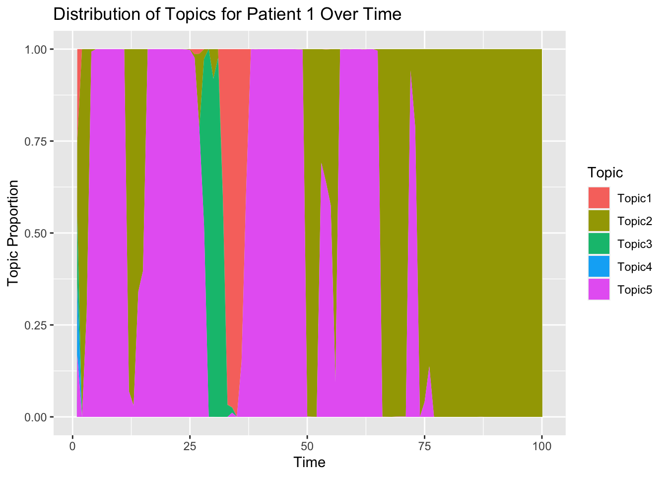
}5.2 Topic Distribution per patient
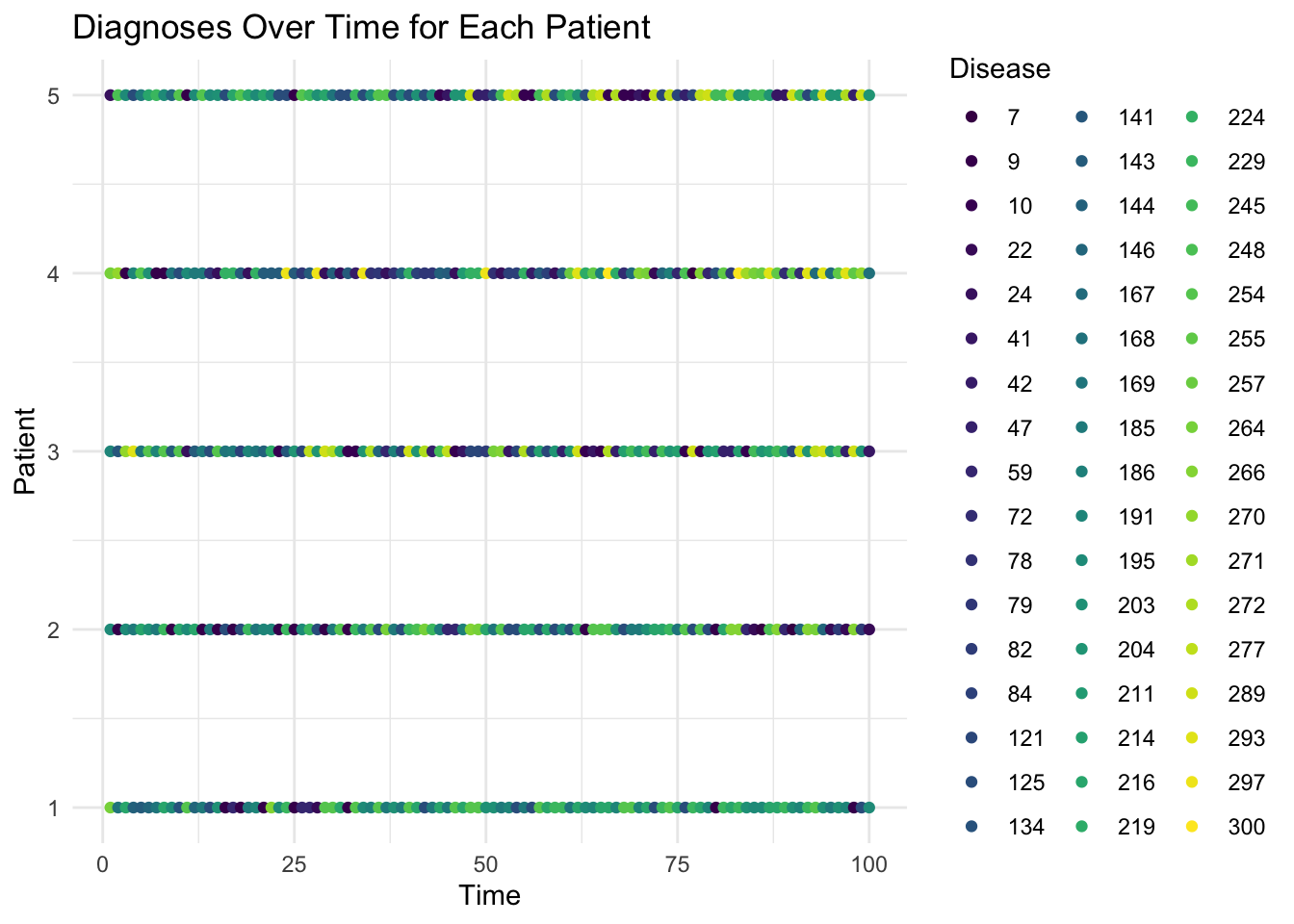
Now let’s select for a sample patient and view his topic distribution over time.
Now, we might want to select a few patients for visualization and watch their disease codes over time.
num_patients=5
num_time_points=100
phi_array=phi

library(ggplot2)

# Function to simulate diagnoses
simulate_diagnoses <- function(theta, phi, num_patients, num_diseases, num_time_points) {
  diagnosis_record <- matrix(NA, nrow = num_patients, ncol = num_time_points)

  for (i in 1:num_patients) {
    for (t in 1:num_time_points) {
      # Aggregate disease probabilities across topics based on patient's theta
      disease_probabilities <- colSums(sweep(phi[, , t], 1, theta[i, , t], '*'))
      # Normalize probabilities
      disease_probabilities <- disease_probabilities / sum(disease_probabilities)
      # Simulate diagnosis
      diagnosed_disease <- sample(1:num_diseases, 1, prob = disease_probabilities)
      diagnosis_record[i, t] <- diagnosed_disease
    }
  }
  return(diagnosis_record)
}

# Assuming theta is indexed as [N, K, T]

library(ggplot2)
library(reshape2)

# Function to simulate diagnoses
simulate_diagnoses <- function(theta, phi, num_patients, num_diseases, num_time_points) {
  diagnosis_record <- matrix(NA, nrow = num_patients, ncol = num_time_points)

  for (t in 1:num_time_points) {
    for (i in 1:num_patients) {
      # Aggregate disease probabilities across topics based on patient's theta at time t
      disease_probabilities <- colSums(sweep(phi[, , t], 1, theta[t, i, ], '*'))
      # Normalize probabilities
      disease_probabilities <- disease_probabilities / sum(disease_probabilities)
      # Simulate diagnosis
      diagnosed_disease <- sample(1:num_diseases, 1, prob = disease_probabilities)
      diagnosis_record[i, t] <- diagnosed_disease
    }
  }
  return(diagnosis_record)
}

# Parameters
num_patients <- 5

# Simulate diagnoses
diagnosis_record <- simulate_diagnoses(theta_over_time, phi, num_patients, V, T)

# Convert to long format for plotting
diagnosis_data_long <- melt(diagnosis_record, varnames = c("Patient", "Time"), value.name = "Disease")

# Plotting
ggplot(diagnosis_data_long, aes(x = Time, y = Patient, color = as.factor(Disease))) +
  geom_point() +
  scale_color_viridis_d() +
  labs(title = "Diagnoses Over Time for Each Patient", x = "Time", y = "Patient", color = "Disease") +
  theme_minimal()