Chapter 4 Adding a time element
Now, in McVean et al, instead of having only one V vector with N_{i} sparse indicators in \(\phi_k\) per topic, there are \(\phi_{kt}\) for a time and topic specific diagnosis distribution.
Easy enough! Recall before we had a matrix that was KxV for the disease distribution per topic.
Now we will initialize an array that is KxVxT that has a disease distribution per topic per time.
The trick is that these need to be somewhat continuous – you can’t go from a 100% probability of hypertension to 0 overnight.
So … they use a natural spline. Here, we introduce a scaled bspline basis (with a knot at 0.5 and 3 degrees) that is scaled by the \(\phi\) we just described inorder to introduce both continuity and preserve sparsity.
The ratio of alpha values influences the relative concentration or preference for certain categories over others. A higher alpha value for a specific category (or categories) relative to others indicates a stronger prior belief or higher expected probability for that category.
4.1 Reviewing Alpha
4.1.1 Ratio of Alpha Values:
The ratio of alpha values influences the relative concentration or preference for certain categories over others. A higher alpha value for a specific category (or categories) relative to others indicates a stronger prior belief or higher expected probability for that category.
4.1.2 Absolute Values of Alpha Parameters:
When all alpha values are greater than 1 (e.g., some are 100 and others are 1), the distribution tends to be more concentrated around the mean, which is influenced by the alpha values. This creates a distribution where most of the probability mass is centered around certain categories (those with higher alpha values).
When alpha values are low (e.g., 1 and 0.01), the distribution is more spread out, and there’s a greater chance of observing more extreme proportions in the categories. Even though the ratio is the same, the overall distribution is less peaked and more variable because the absolute values are smaller.
4.1.3 Interpretation in our Context:
Alpha = 100 vs. Alpha = 1: This setup indicates a strong prior belief in the topic-specific diseases (with alpha = 100) compared to non-topic-specific diseases. The distribution will be quite peaked around these topic-specific diseases, meaning that most of the probability mass is concentrated there.
Alpha = 1 vs. Alpha = 0.01: Although the relative preference for topic-specific diseases over non-topic-specific diseases is the same (in terms of ratio), the overall distribution will be more spread out. This means that while there’s a preference for topic-specific diseases, the probabilities are not as heavily concentrated around them as in the first scenario.
K <- 5  # Number of topics
V <- 300  # Number of diagnoses
T <- 100            # Number of time points
time_points <- seq(0, 100, length.out = T)
phi <- array(dim = c(K, V, T))

for (k in 1:K) {
    for (v in 1:V) {
        # Assign higher probabilities to certain diseases for each topic
        # Placeholder: Assigning higher weights to some diseases
        if (v%in%topic_spec_disease[k,]) {
          print(v)
            beta[v] <- V ### make spiky and will be close to 1/d then
        } else {
            beta[v] <- 1
        }
    }
    phi[k,,1] <- rdirichlet(1, beta)
}
## [1] 72
## [1] 141
## [1] 167
## [1] 168
## [1] 219
## [1] 255
## [1] 257
## [1] 270
## [1] 293
## [1] 300
## [1] 10
## [1] 41
## [1] 47
## [1] 121
## [1] 204
## [1] 214
## [1] 245
## [1] 272
## [1] 277
## [1] 289
## [1] 9
## [1] 125
## [1] 169
## [1] 185
## [1] 191
## [1] 195
## [1] 203
## [1] 216
## [1] 229
## [1] 254
## [1] 24
## [1] 42
## [1] 78
## [1] 79
## [1] 84
## [1] 143
## [1] 144
## [1] 211
## [1] 224
## [1] 297
## [1] 7
## [1] 22
## [1] 59
## [1] 82
## [1] 134
## [1] 146
## [1] 186
## [1] 248
## [1] 264
## [1] 266#
# # Normalize initial phi
# for (k in 1:K) {
# phi[k, , 1] <- phi[k, , 1] / sum(phi[k, , 1])
# }
summary(rowSums(phi[,,1]))## Min. 1st Qu. Median Mean 3rd Qu. Max.
## 1 1 1 1 1 1## [[1]]
## Min. 1st Qu. Median Mean 3rd Qu. Max.
## 0.08188 0.08702 0.09293 0.09168 0.09616 0.10128
##
## [[2]]
## Min. 1st Qu. Median Mean 3rd Qu. Max.
## 0.08514 0.08850 0.08967 0.09008 0.09077 0.09550
##
## [[3]]
## Min. 1st Qu. Median Mean 3rd Qu. Max.
## 0.08167 0.08753 0.09386 0.09143 0.09539 0.09678
##
## [[4]]
## Min. 1st Qu. Median Mean 3rd Qu. Max.
## 0.08495 0.08984 0.09103 0.09105 0.09263 0.09815
##
## [[5]]
## Min. 1st Qu. Median Mean 3rd Qu. Max.
## 0.08331 0.08822 0.09095 0.09082 0.09398 0.09867## [[1]]
## Min. 1st Qu. Median Mean 3rd Qu. Max.
## 2.370e-06 7.863e-05 1.958e-04 3.344e-03 4.205e-04 1.013e-01
##
## [[2]]
## Min. 1st Qu. Median Mean 3rd Qu. Max.
## 3.470e-06 1.111e-04 2.699e-04 3.344e-03 4.931e-04 9.550e-02
##
## [[3]]
## Min. 1st Qu. Median Mean 3rd Qu. Max.
## 5.000e-08 9.182e-05 2.135e-04 3.343e-03 4.255e-04 9.678e-02
##
## [[4]]
## Min. 1st Qu. Median Mean 3rd Qu. Max.
## 5.800e-07 9.879e-05 2.286e-04 3.344e-03 4.558e-04 9.815e-02
##
## [[5]]
## Min. 1st Qu. Median Mean 3rd Qu. Max.
## 3.900e-07 8.638e-05 2.147e-04 3.344e-03 4.442e-04 9.867e-02all_normalized <- all(apply(phi[, , 1], 1, function(x) abs(sum(x) - 1) < .Machine$double.eps^0.5))
print(all_normalized) # Should print TRUE if all are normalized## [1] TRUEdegree=3
knots=0.5
## in McVean they have a set of spline functions across time for each of the KxV diseases, so we choose each set of coefficients randomly for each disease
# Apply spline transformation with positive coefficients
for (k in 1:K) {
for (v in 1:V) {
# First, generate a disease specific B-spline basis
bspline_basis <- bs(time_points, knots = knots, degree = degree, intercept = TRUE)
# Generate positive coefficients for the spline, ensuring they are small enough
# to not dominate the topic-specific diseases
coef <- runif(length(knots) + degree + 1, min = 0, max = 0.5)
# Calculate spline values ensuring they are non-negative
spline_values <- bspline_basis %*% coef
# For topic-specific diseases, scale the spline values based on initial phi
# For non-topic-specific diseases, dampen the effect to keep them low
if (v %in% topic_spec_disease[k,]) {
scaled_spline_values <- spline_values * phi[k, v, 1] / max(spline_values)
} else {
# Apply a dampening factor to non-topic specific diseases
dampening_factor <- 0.01
scaled_spline_values <- spline_values * dampening_factor * phi[k, v, 1] / max(spline_values)
}
# Store the scaled spline values
phi[k, v, ] <- scaled_spline_values
}
}
matplot(bspline_basis)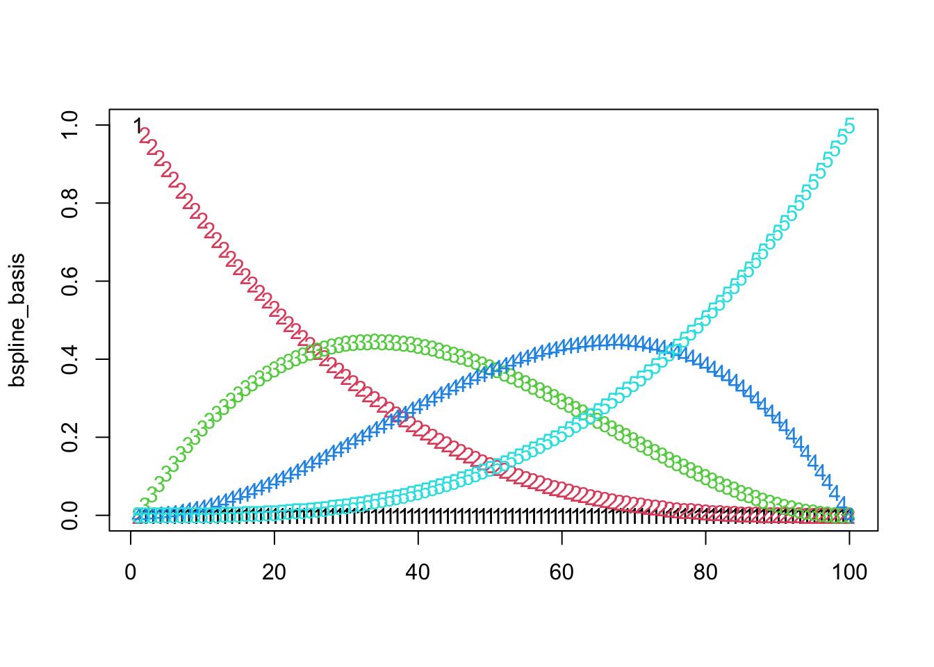
4.2 Normalization
We need to normalize phi over time after this spline transfomration to ensure a proper distribution:
# Normalize phi over time after spline transformation
for (t in 1:T) {
for (k in 1:K) {
sum_phi_kt <- sum(phi[k, , t])
if (sum_phi_kt > 0) {
phi[k, , t] <- phi[k, , t] / sum_phi_kt
}
}
}
# Check normalization for each time point
all_normalized <- TRUE
for (t in 1:T) {
if (!all(apply(phi[, , t], 1, function(x) abs(sum(x) - 1) < .Machine$double.eps^0.5))) {
all_normalized <- FALSE
break
}
}
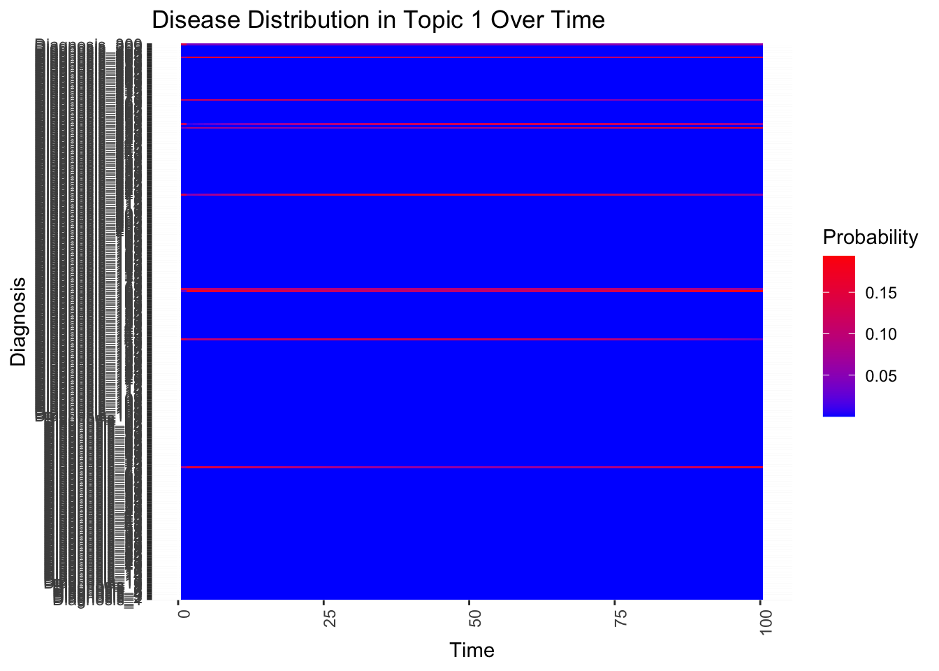
print(all_normalized) # Should print TRUE if all are normalized```## [1] TRUENow \(\phi\) is the array of diseases x topics x time, so for a given topic, this should be continous. Let’s look at a sample topic with a few diseases to check:
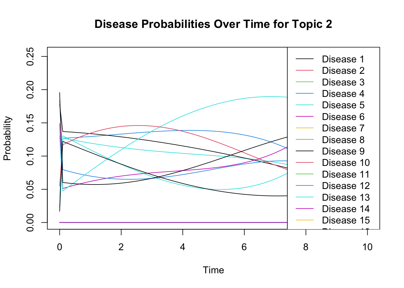
We can see that this corresponds with the disease we’ve chosen in topic_disease.