Chapter 3 Simulation of Topic Weights
To simulate topic weights over time, we utilize a logistic growth function with parameters influenced by individual-specific genetic predispositions (gamma). The topic weights (Theta) evolve according to a logistic function that ensures lower activity at early ages and higher activity as time progresses.
3.0.1 Apply \(\gamma\) to Modulate the Rate of Change:
After generating the GP paths, you can modulate these paths using \(\gamma\) to reflect individual-specific rates of change in topic probabilities, accommodating the genetic predisposition aspect
3.1 We first observe the data to try and choose the right structure of our mean fucntion
So whcih fits the data?
##
## Attaching package: 'dplyr'
## The following objects are masked from 'package:stats':
##
## filter, lag## The following objects are masked from 'package:base':
##
## intersect, setdiff, setequal, union##
## Attaching package: 'reshape2'## The following object is masked from 'package:tidyr':
##
## smiths##
## Attaching package: 'MASS'## The following object is masked from 'package:dplyr':
##
## selectlibrary(ggsci)
# d=readRDS("~/Dropbox/groupdata.rds")
# # Plot histogram
# ggplot(d, aes(x = age, y = length, fill = group)) +
# geom_histogram(stat = "identity", position = "dodge") +
# facet_wrap(~group, scales = "free_y") +
# labs(title = "Frequency of Diagnoses by Age",
# x = "Age",
# y = "Frequency",
# fill = "Group") +
# theme_minimal()
dp=readRDS("dplot.rds")
dp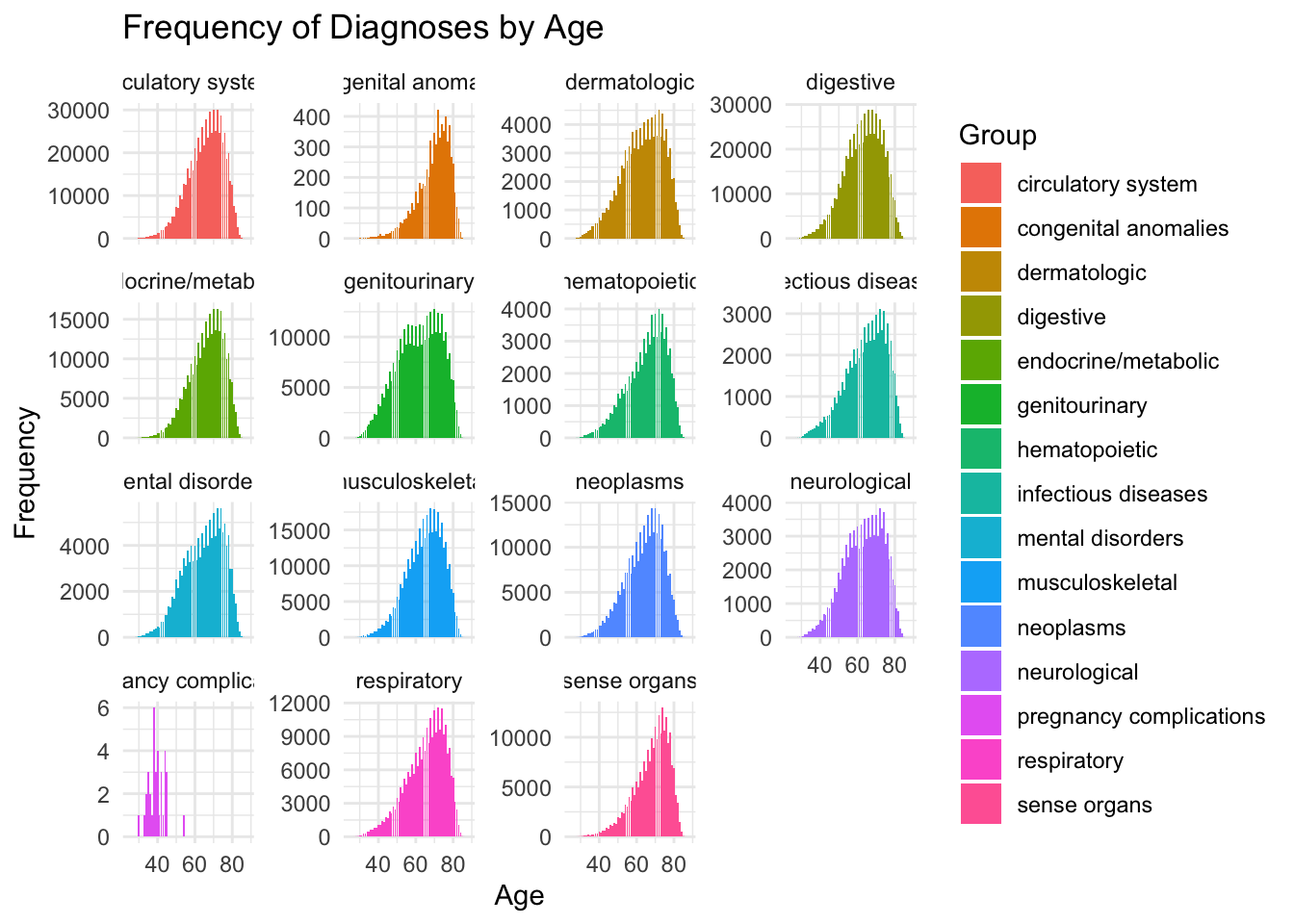
We see that for most topics, the age of incidence is monotonically increasing. We want a funciton that does this – so we simulate our GP with different logistic mean functions.
We could use a markov model, but the exponential growth in the number of possible topic combinations as the number of topics increases is a significant challenge when using a Hidden Markov Model (HMM) to directly model topic combinations.
3.2 Why Independent Topic Modeling is Advantageous
Scalability: By modeling each topic independently, you avoid the exponential explosion of states that would occur if you were to model all possible combinations of topics. This makes the model much more computationally tractable, especially as the number of topics increases.
Interpretability: Independent topic modeling allows you to interpret the effect of genetic predisposition and temporal dynamics on each topic separately. This can provide clearer insights into the factors influencing the activation of specific topics.
Flexibility: The GP framework allows for flexible modeling of the temporal dynamics of each topic, capturing smooth trends, correlations between time points, and individual-specific variations.
3.3 Logistic
If we want to adjust the Gaussian Process (GP) to make the topics less likely to be active early on and to gradually increase their activity over time, we can modify the mean function
\(\mu(t)\) of the GP to introduce a logistic growth curve instead of a linear one. This logistic growth curve will start with lower values (representing lower activity) and asymptotically approach a higher value (representing higher activity) as time progresses.
However, if we know the topic activity is lower at early ages we might want to simply use a logistic function. We allow the genetic parameter \(\gamma\) to influence the mean shift.
We don’t necessarily need the noise of the gaussian process here, we can just have it evolve smoothly according ato a logistic function since we know that topic occurrence tends to increase with time:
# Parameters
D <- 20  # Number of individuals
K <- 5   # Number of topics
T <- 100  # Number of time points
V=50
time_points <- 1:T

# Individual and topic-specific gamma values
gamma <- matrix(runif(D * K, min = 0.5, max = 2), nrow = D, ncol = K)

# Function to create modified logistic growth mean
create_modified_logistic_mean <- function(time_points, mid_point, max_value, growth_rate, gamma) {
  s <- (gamma*max_value) / (1 + exp(-growth_rate * (time_points - mid_point)))
  s <- s * (1 - exp(-0.1 * time_points)) # Ensure lower activity at early ages
  return(s)
}

# Generate logistic curves for each topic and individual
mu_population <- matrix(0, nrow = K, ncol = T)
mid_points <- runif(K, 50, 80)
max_values <- runif(K, 0.2, 0.8)
growth_rates <- runif(K, 0.05, 0.2)

for (k in 1:K) {
  mu_k <- create_modified_logistic_mean(time_points, mid_points[k], max_values[k], growth_rates[k], 1)
  mu_population[k, ] <- mu_k
}

# Generate individual-specific topic distributions
Theta_individual <- array(dim = c(D, K, T))
Theta_pop <- array(dim = c(K, T))
Topic_activity <- array(dim = c(D, K, T))

for (d in 1:D) {
  for (k in 1:K) {
    # Adjust the logistic mean curve for this individual's predisposition
      Theta_pop[ k, ] <- create_modified_logistic_mean(time_points, mid_points[k], max_values[k], growth_rates[k], 1)

    predisposition_score_dk <- gamma[d, k]
    adjusted_mu_k <- create_modified_logistic_mean(time_points, mid_points[k], max_values[k], growth_rates[k], predisposition_score_dk)

    # Add noise to introduce variability
    #noise <- rnorm(T, mean = 0, sd = 0.05)
    noise=rep(0,T)# Adjust the standard deviation as needed
    noisy_mu_k <- adjusted_mu_k + noise

    # Ensure the values are between 0 and 1
    noisy_mu_k <- pmin(pmax(noisy_mu_k, 0), 1)
    Theta_individual[d, k, ] <- noisy_mu_k
    Topic_activity[d, k, ] <- rbinom(T, 1, noisy_mu_k)
  }
}
# Create a data frame for plotting
melt_topic_activity <- function(activity_array) {
activity_df <- melt(activity_array)
names(activity_df) <- c("Individual", "Topic", "Time", "Activity")
activity_df$Active <- ifelse(activity_df$Activity == 1, paste("Active", activity_df$Topic), "Inactive")
return(activity_df)
}
df <- melt_topic_activity(Topic_activity)
# Define color palette
num_active_levels <- length(setdiff(unique(df$Active), "Inactive"))
softer_palette <- brewer.pal(min(num_active_levels, 8), "Set2") # Use Set2 palette for up to 8 different active levels
active_levels <- setdiff(unique(df$Active), "Inactive")
colors_for_active <- setNames(softer_palette[1:num_active_levels], active_levels)
colors <- c("Inactive" = "white", colors_for_active)
# Plotting functions
plot_population <- function(df) {
ggplot(df, aes(x = Time, y = Topic, fill = Active)) +
geom_tile() +
scale_fill_manual(values = colors) +
labs(title = "Population-Level Topic Activity Over Time",
x = "Time", y = "Topic", fill = "Topic Status") +
theme_minimal() +
theme(axis.text.x = element_text(angle = 90, hjust = 1),
legend.position = "bottom")
}
plot_individual <- function(df, individual_id) {
individual_df <- df %>% filter(Individual == individual_id)
ggplot(individual_df, aes(x = Time, y = as.factor(Topic), fill = Active)) +
geom_tile() +
scale_fill_manual(values = colors) +
labs(title = paste("Topic Activity Over Time for Individual", individual_id),
x = "Time", y = "Topic", fill = "Topic Status") +
theme_minimal() +
theme(axis.text.x = element_text(angle = 90, hjust = 1),
legend.position = "bottom")
}
plot_high_predisposition <- function(df, individual_id) {
high_predisposition_df <- df %>% filter(Individual == individual_id)
ggplot(high_predisposition_df, aes(x = Time, y = as.factor(Topic), fill = Active)) +
geom_tile() +
scale_fill_manual(values = colors) +
labs(title = paste("High Predisposition Individual", individual_id, "Topic Activity Over Time"),
x = "Time", y = "Topic", fill = "Topic Status") +
theme_minimal() +
theme(axis.text.x = element_text(angle = 90, hjust = 1),
legend.position = "bottom")
}
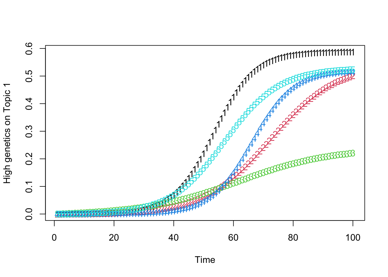
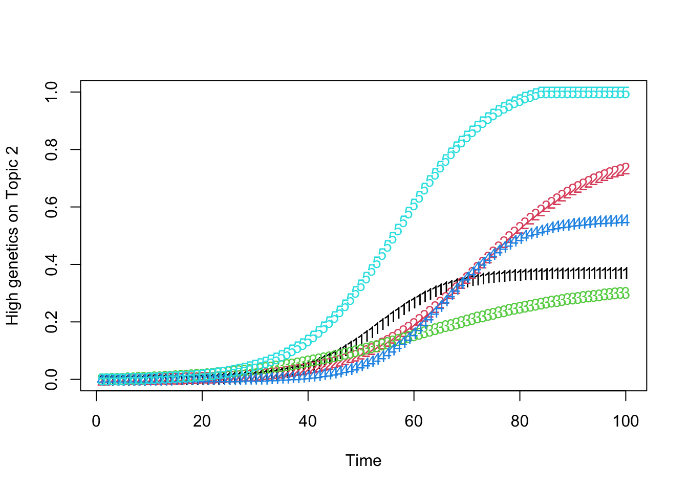
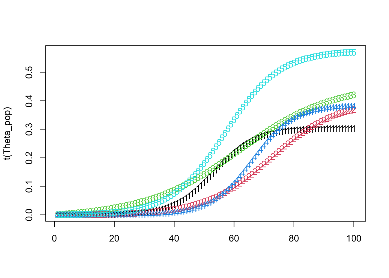
matplot(t(Theta_pop))

plot_low_predisposition <- function(df, individual_id) {
  high_predisposition_df <- df %>% filter(Individual == individual_id)
  ggplot(high_predisposition_df, aes(x = Time, y = as.factor(Topic), fill = Active)) +
    geom_tile() +
    scale_fill_manual(values = colors) +
    labs(title = paste("Low Predisposition Individual", individual_id, "Topic Activity Over Time"),
         x = "Time", y = "Topic", fill = "Topic Status") +
    theme_minimal() +
    theme(axis.text.x = element_text(angle = 90, hjust = 1),
          legend.position = "bottom")
}

# Identify individuals with high and low genetic predispositions
high_predisposition_individual <- which.max(rowSums(gamma))
low_predisposition_individual <- which.min(rowSums(gamma))

# 1. Population-Level Topic Activity
print(plot_population(df))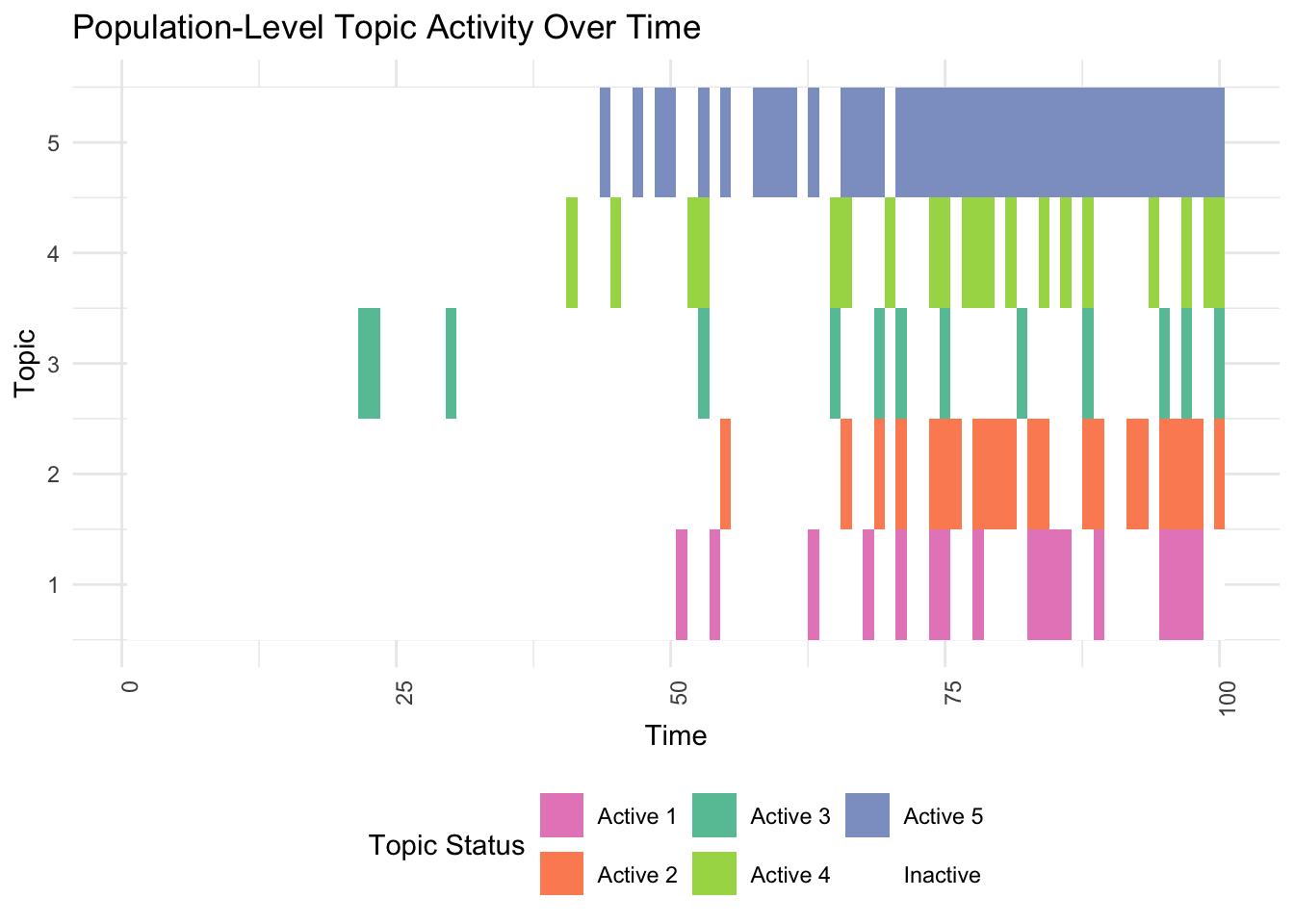
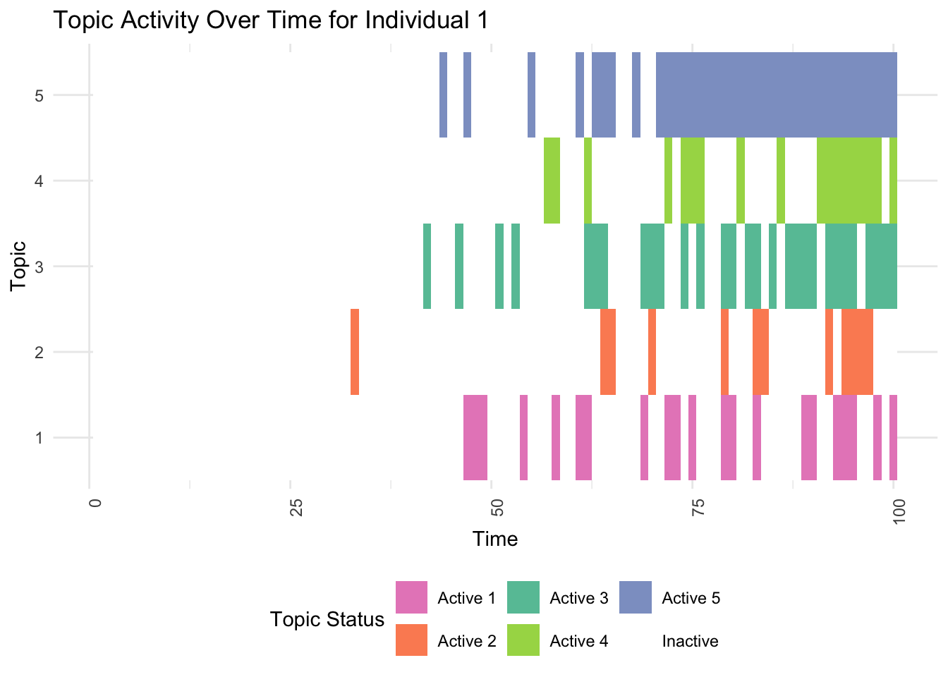
# 3. Detailed View for an Individual with High Predispositions
print(plot_high_predisposition(df, high_predisposition_individual))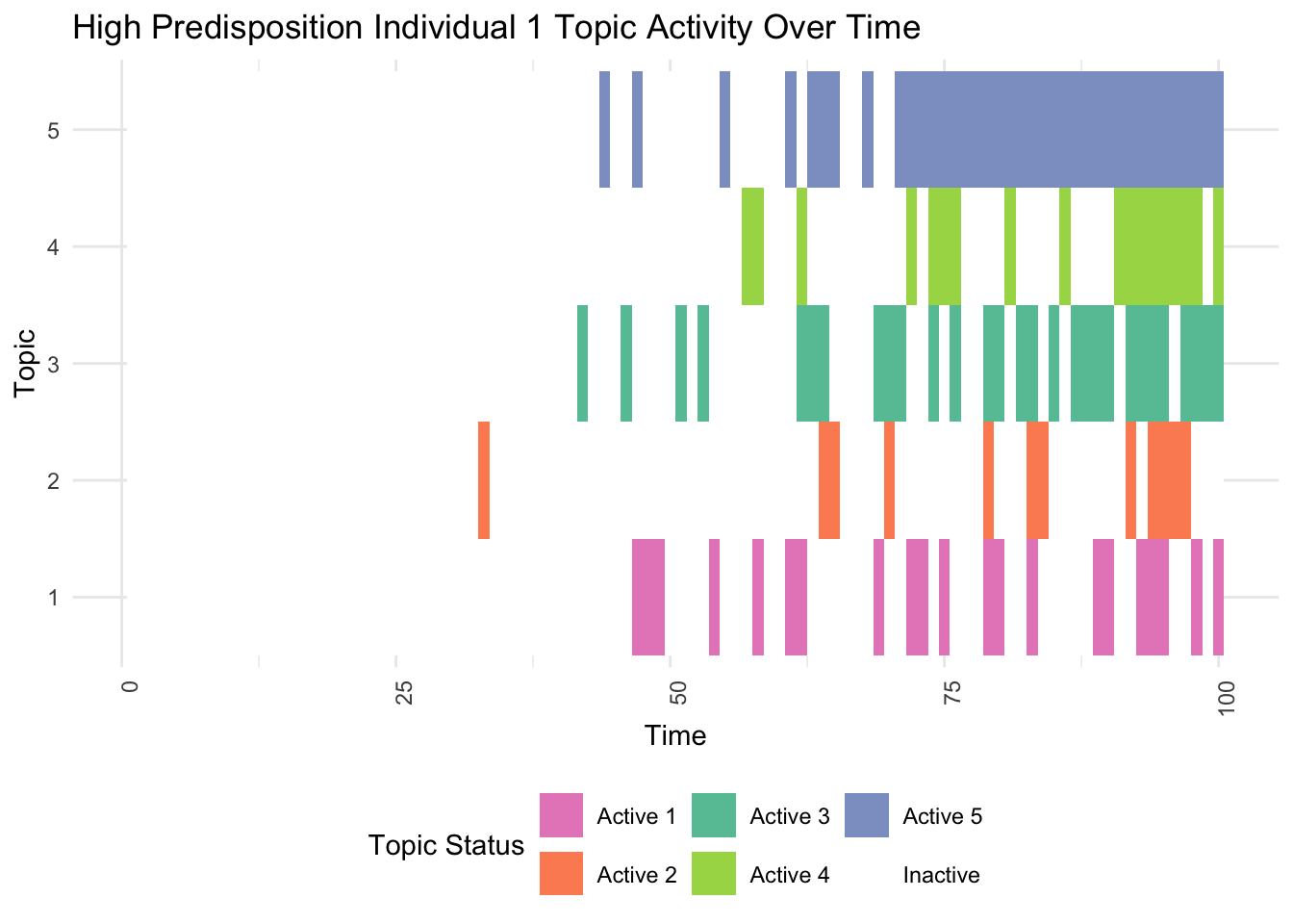
# 4. Detailed View for an Individual with Low Predispositions
print(plot_low_predisposition(df, low_predisposition_individual))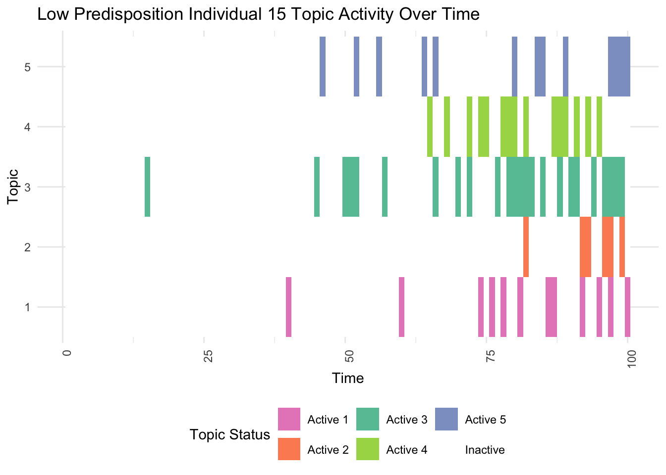
Plot theta
mf=melt(Theta_individual)
colnames(mf)=c("Individual","Topic","Time","Value")
ggplot(mf[mf$Individual%in%sample(D,1),],aes(x=Time,y=Value,group=as.factor(Topic),fill=as.factor(Topic)))+geom_area()+theme_classic()+labs(y="Theta",x="Age")+scale_fill_nejm()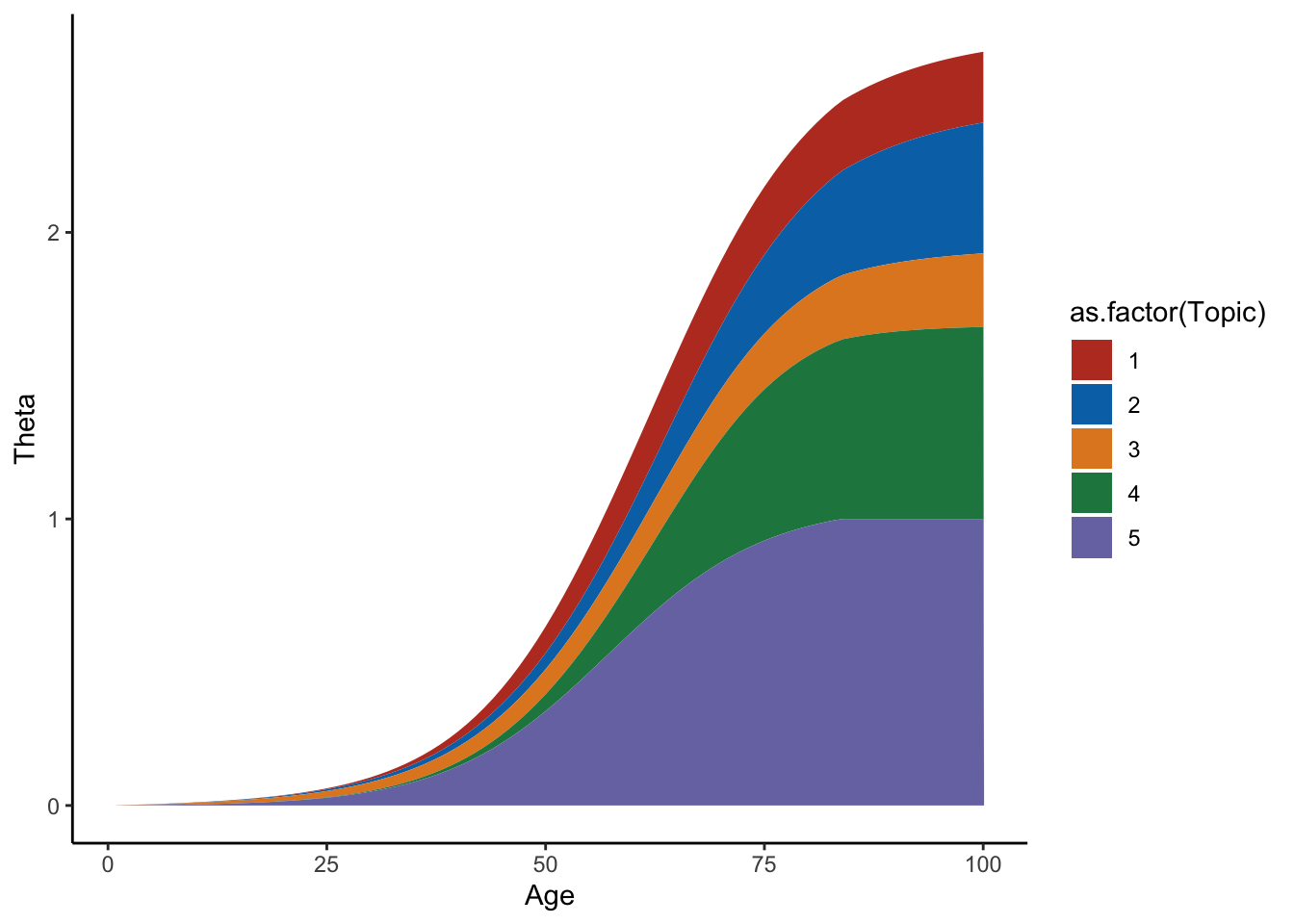
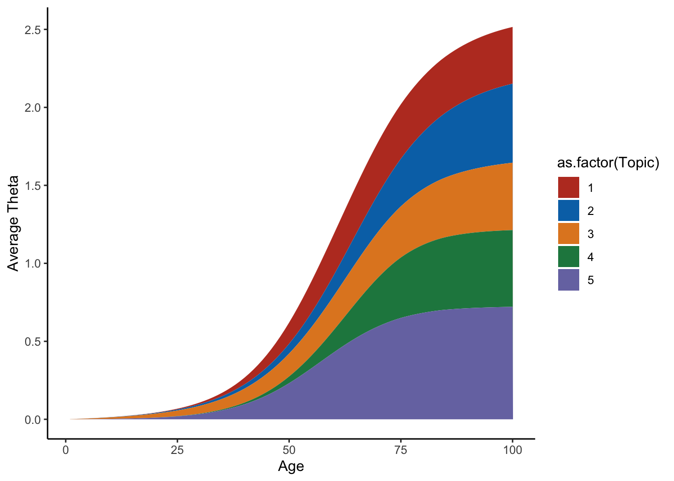
average=apply(Theta_individual,c(2,3),mean)
m=melt(average)
colnames(m)=c("Topic","Time","Value")
ggplot(m,aes(x=Time,y=Value,group=Topic,fill=as.factor(Topic)))+geom_area()+theme_classic()+labs(y="Average Theta",x="Age")+scale_fill_nejm()