Chapter 4 Simulation of Disease Loadings
For the disease loadings, we use different mean functions to simulate the progression of disease probabilities over time. We assume that diseases tend to be topic-specific and heavily loaded on a few topics.
cov_function <- function(t1, t2, lengthscale, variance) {
    exp(-0.5 * (t1 - t2)^2 / lengthscale^2) * variance
}

# Store disease-specific covariances
Sigma <- array(dim = c(K, V, T, T)) # K topics, V diseases, T x T covariance matrix each


eta <- array(dim = c(K, V, T))


# Bias factor (adjust as needed)


# Generate covariances (adjust as needed)
for (k in 1:K) {
  for (v in 1:V) {
    # Sample a single lengthscale and variance for each topic-disease pair
      cov_matrix_kv <- matrix(0, nrow = T, ncol = T)
      #lengthscale_kv <- runif(1,min=5,max=20) ## choose random lengthscale for each topic and disease
      #variance_kv <- runif(1,0.1,0.5)## choose random variance for each topic and disease
      variance_kv=0.01 ## smaller variance means it changes less from mu funciotn

      lengthscale_kv=10
    for (i in 1:T) {
for (j in 1:T) {
        cov_matrix_kv[i, j] <- cov_function(i, j, lengthscale_kv, variance_kv)
      }
    }

    Sigma[k, v, , ] <- cov_matrix_kv
  }
}
4.1 Sample from the Gaussian Process
The probability of a disease within a topic over time has some covariance structure. We also might imagine that the disease probabilities also have some shape over time:
linear_trend <- function(time,
                         slope = 0.1,
                         intercept = 0) {
  return(slope * time + intercept)
}


logistic_growth <-
  function(t, carrying_capacity, growth_rate, t_mid) {
    carrying_capacity / (1 + exp(-growth_rate * (t - t_mid)))
  }


exponential_decay <- function(t, initial_value, decay_rate) {
  initial_value * exp(-decay_rate * t)
}

gaussian_peak <- function(t, mean, variance) {
  exp(-(t - mean) ^ 2 / (2 * variance))
}


polynomial_trend <- function(t, coefficients) {
  result <- sapply(t, function(time_point) {
    sum(sapply(1:length(coefficients), function(i) coefficients[i] * time_point^(i - 1)))
  })
  return(result)
}

sinusoidal_pattern <- function(t, amplitude, period, phase) {
  amplitude * sin((2 * pi / period) * t + phase)
}

cov_function <- function(t1, t2, lengthscale, variance) {
  return(variance * exp(-0.5 * (t1 - t2) ^ 2 / lengthscale ^ 2))
}
We might wish that each disease within a topic ihas it’s unique mean function:
# Modify eta sampling to use the correct covariance
# Covariance matrix Sigma (you should define this according to your model specifics)
# Parameters

D <- 20  # Number of individuals
K <- 5   # Number of topics
T <- 100  # Number of time points
time_points <- 1:T

# Initialize the array
topic_word_mean <- array(NA, dim = c(K, V))


mean_functions <- list(
  linear_trend = linear_trend,
  logistic_growth = logistic_growth,
  #exponential_decay = exponential_decay,
  gaussian_peak = gaussian_peak
  #polynomial_trend = polynomial_trend
  #sinusoidal_pattern = sinusoidal_pattern
)

# Define a list of names for the mean functions
mean_function_names <- names(mean_functions)


# Simulate mean functions for each disease
mu_vectors <- list()
mean_functions_called = list()


for (k in 1:K) {
  mu_vectors[[k]] <- list()
  mean_functions_called[[k]] = list()
  for (v in 1:V) {
    # Choose a mean function randomly
    # Choose a mean function by name randomly
    chosen_function_name <- sample(mean_function_names, 1)
    # Retrieve the function from the list using the name
    mean_function <- mean_functions[[chosen_function_name]]
    # Sample parameter ranges
 params <- list(
      slope = runif(1, -0.05, 0.05),
      intercept = runif(1, -1, 1),
      carrying_capacity = runif(1, 0.02, 0.05),
      growth_rate = runif(1, 0.01, 0.05),
      t_mid = sample(time_points, 1),
      mean = sample(time_points, 1),
      variance = runif(1, 10, 50),
      coefficients = runif(3, -0.1, 0.1)
    )


    # Use the appropriate parameters based on the chosen mean function
    if (chosen_function_name  == "logistic_growth") {
      function_specific_params <- list(
        t = time_points,
        carrying_capacity = params$carrying_capacity,
        growth_rate = params$growth_rate,
        t_mid = params$t_mid
      )
    } else if (chosen_function_name  == "linear_trend") {
      function_specific_params <- list(
        t = time_points,
        slope = params$slope,
        intercept = params$intercept
      )
    } else if (chosen_function_name  == "exponential_decay") {
      function_specific_params <- list(
        t = time_points,
        initial_value = params$initial_value,
        decay_rate = params$decay_rate
      )
    } else if (chosen_function_name  == "gaussian_peak") {
      function_specific_params <- list(t = time_points,
                                       mean = params$mean,
                                       variance = params$variance)
    } else if (chosen_function_name == "polynomial_trend") {
      function_specific_params <- list(t = time_points, coefficients = params$coefficients)
    } else if (chosen_function_name  == "sinusoidal_pattern") {
      function_specific_params = list(
        t = time_points,
        amplitude = params$amplitude,
        period = params$period,
        phase = params$phase
      )
    }


    # Generate the time series for the mean function using do.call
    mu_vectors[[k]][[v]] <-
      do.call(mean_function, function_specific_params)
    mean_functions_called[[k]][[v]] = list("function_name" = chosen_function_name, "params" = function_specific_params)

    eta[k, v, ] <-
      mvrnorm(1, mu = mu_vectors[[k]][[v]], Sigma = Sigma[k, v, , ])
  }
}


rho = matrix(runif(K*D,min = 0.5,max = 2),nrow=D,ncol=K)
#rho=matrix(1,nrow=D,ncol=K)
# Normalize using logistic function and a scaling factor
adjusted_logistic_function <- function(x, scale) {
  return(scale / (1 + exp(-x)))
}


inv_time_warping <- function(t, rho, T) {
return(min(T, max(1, floor((t / T) ^ (1 / rho) * T))))
}


# Initialize inverse warped time array
inv_warped_t_array <- array(0, dim = c(D, K, T))

for (d in 1:D) {
  for (k in 1:K) {
    for (t in 1:T) {
      inv_warped_t_array[d, k, t] <- inv_time_warping(t, rho[d, k], T)
    }
  }
}
4.2 Topic specificity
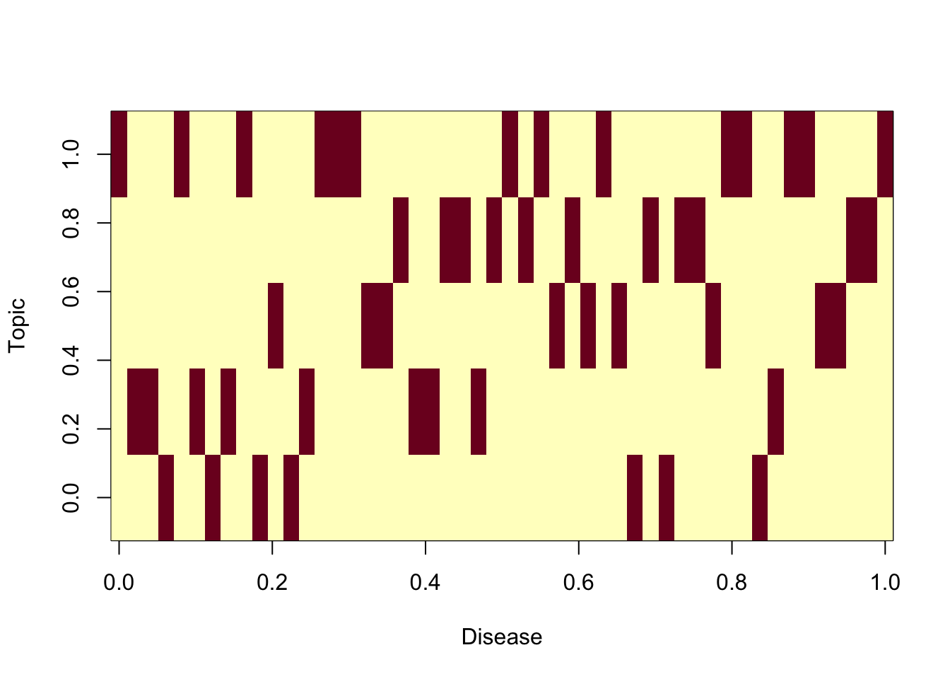
We simiulate so that disease tend to be somewhat topic specific, that is, heavilty loaded on a few topics
# Determine the number of topics in which each disease will be primarily active
#num_topics_per_disease <- sample(1:2, V, replace = TRUE)  # Each disease is active in 1 or 2 topics
num_topics_per_disease = rep(1,V)
# Initialize the list to store the primary topics for each disease
disease_primary_topics <- vector("list", length = V)

# Initialize the disease-topic matrix with zeros indicating inactivity
disease_topic_matrix <- matrix(0, nrow = V, ncol = K)

# Assign primary topics to each disease
for (disease in 1:V) {
  primary_topics <- sample(1:K, num_topics_per_disease[disease])
  disease_primary_topics[[disease]] <- primary_topics

  # Set the bias value for the disease in its primary topics, can vary
  #bias_values <- runif(num_topics_per_disease[disease], 0, 1)  # Variable bias between 0 and 1
  bias_values = rep(1,num_topics_per_disease[disease])
  # Fill in the disease-topic matrix with bias values for the primary topics
  disease_topic_matrix[disease, primary_topics] <- bias_values
}


image(t(disease_topic_matrix),xlab="Topic",ylab="Disease")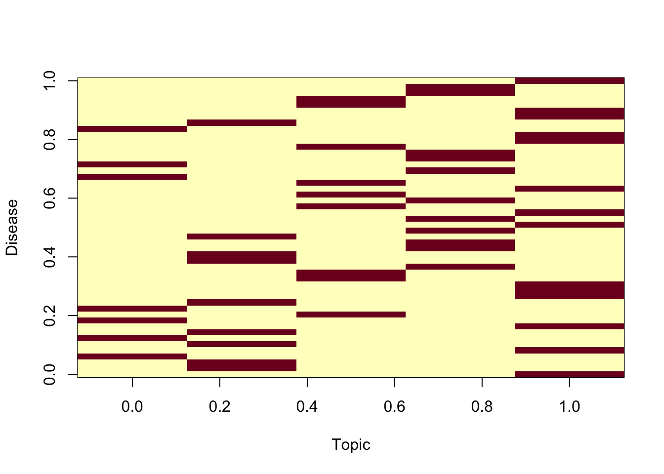
4.3 Now do on population for different warping
beta <- array(0, dim(eta))
# Normalize using logistic function and a scaling factor
adjusted_logistic_function <- function(x, scale) {
  return(scale / (1 + exp(-x)))
}

scaling_factor <- 0.02  #

bias_value=max(eta)
for (topic_idx in 1:K) {
    # Retrieve the diseases and their risk periods for this topic
    #specific_diseases_periods <- topic_disease_risk_periods[[topic_idx]]
    bias_increase <- disease_topic_matrix[,topic_idx]*bias_value
    for (time_idx in 1:T) {

      disease_values <- eta[topic_idx, , time_idx]

      # Increase the values for active diseases at this time before normalization
      dv <- disease_values+bias_increase

      # Apply softmax normalization
      normalized_disease <- adjusted_logistic_function(dv,scale = scaling_factor)
            #normalized_disease <- softmax_normalize(dv)

      beta[topic_idx, , time_idx] <- normalized_disease
    }
}
Show that disease probabilities for two people of different \(\rho\):
v=sample(topic_specific_diseases[[topic_idx]],1)
plot(beta[topic_idx,v,],pch=19,col="grey",ylab="Disease Probability over Time conditional on topic activity",xlab="Time")
t_high=inv_warped_t_array[which.max(rho[,topic_idx]),topic_idx,]
points(seq(1:T),beta[topic_idx,v,t_high],col="red",pch=19)
t_low=inv_warped_t_array[which.min(rho[,topic_idx]),topic_idx,]
points(seq(1:T),beta[topic_idx,v,t_low],col="blue",pch=19)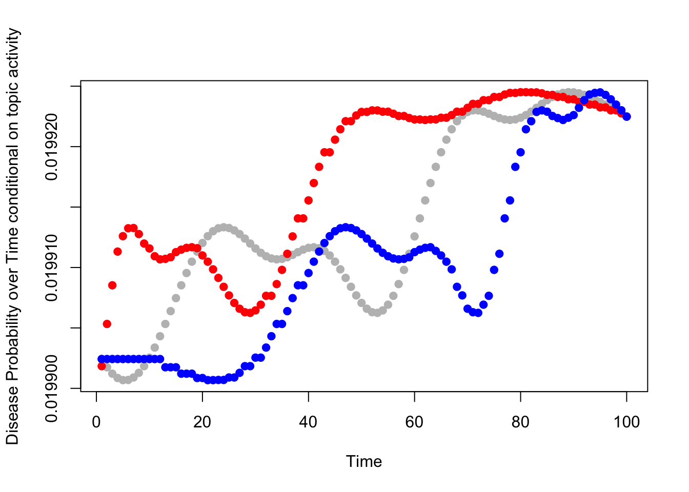
Expand beta_prime array so that it stores the right value for each individual: