Chapter 12 The Machine Learning Pipeline
12.1 Training, validation, and test sets
In supervised learning, the data used to build the final model usually comes from multiple datasets. In particular, three data sets are commonly used in different stages of the creation of the model:
The Training set is a set of examples (i.e. observations) used to fit a learner by minimizing the empirical risk on it. For instance, if our learner is an SVM classifier, than we use the training dataset to learn its weights in a supervised learning framework.
Successively, the fitted model is used to predict the responses for the observations in a second dataset called the validation dataset. The validation dataset provides an unbiased evaluation of a learner fit on the training dataset. We evaluate the performance of the learner over a (potentially) independent dataset in order to do hyper-parameter tuning, variable selection, or model selection. That is, for each type of learner we trained over the training set, we have an independent performance measure. If we believe independence exist, and that the train-validation split generalizes the data distribution in the real world, we can chose the learner with the best score (given some aggregation method) to be the final model. Examples of hyperparameters that we use validation set to tune: k in k-nearest Neighbors, the cost parameter in SVM, the number of hidden layers in deep neural net, the regularization parameters in Elastic net, or the maximal tree depth in Xgboost. The motivation in validate trained models can be seen as: empirically deciding on the appropriate relation between complexity and simplicity. In other words, answering the question: when do we start to overfit the training data.
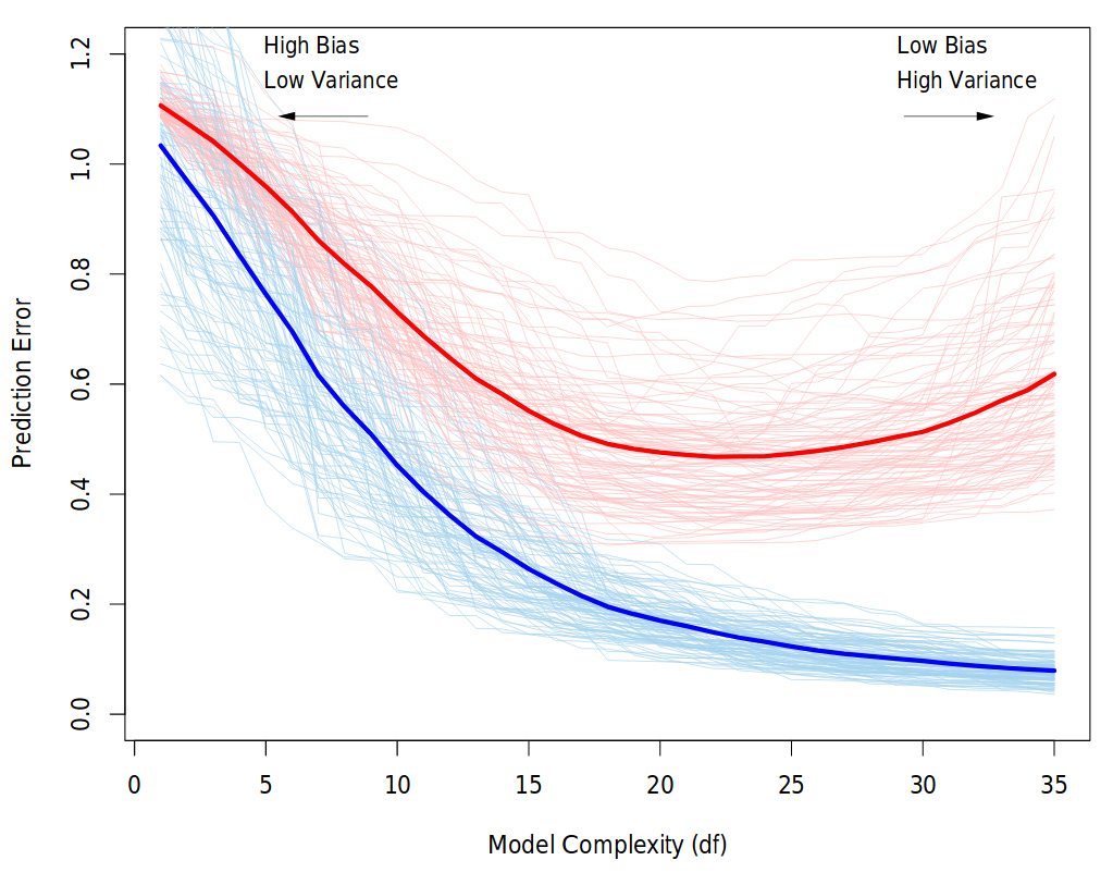
Behavior of validation and training sample error as the model complexity is varied. The light blue and red curves show the training error and the conditional validation error for 100 training sets, as the model complexity is increased. The solid curves show the expected validation and training error. It is clear that from some level, adding more complexity to the model hurts validation performance, while training performance continue to improve. The purpose of the validation phase here is to find the point of the minimum validation error. Source: “The Elements of Statistical Learning” book
Finally, the test dataset is a dataset used to provide an unbiased evaluation of a final model fit on the training dataset. Note: it is important that data from the test set was held out, i.e., has never been used in any of the training phases.
12.2 Cross validation (CV)
Instead of a permanent train-validation splitting, a dataset can be repeatedly split into a training and a validation datasets. This is known as cross-validation (CV). These repeated partitions can be done in various ways.
The most intuitive is the K-fold Cross-validation: The data used for training (all except the test set) is randomly partitioned into k subsamples. Of the k subsamples, a single subsample is retained as the validation set, and the remaining k − 1 subsamples are used for training. The process is then repeated k times, with each of the k subsamples used exactly once as the validation set. All k results are than aggregated.
There are many more CV approaches. Examples are Repeated random sub-sampling; Leave-one-out (LOO); Leave-p-out (LPO); Monte-Carlo; and h-block cross validation.
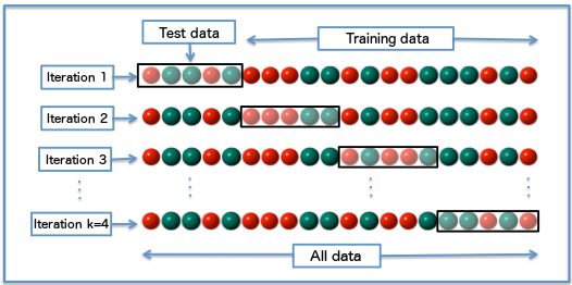
Diagram of k-fold cross-validation with k=4. Source: Wikipedia
We emphasize that CV in dependence setting is not straightforward, and its a gentle art to cross-validate in situations where you can’t shuffle your data, e.g.: time-series data or spatial data.
12.3 What is the Machine Learning Pipeline?
A machine learning typical project can usually be seen as a set of data processing elements connected in series, where the output of one element is the input of the next one. Usually there are some feedbacks between phases in the series, which relate to the learning process. This structure is sometimes referred as a machine learning pipeline. The parallelization structure of the process (i.e., the precise manner in which the computations will be distributed across multiple processing units) is of great importance in the pipeline. However, Explicit Parallelism is beyond the scope of this course and we will rely on the internal parallelization structure of R libraries.
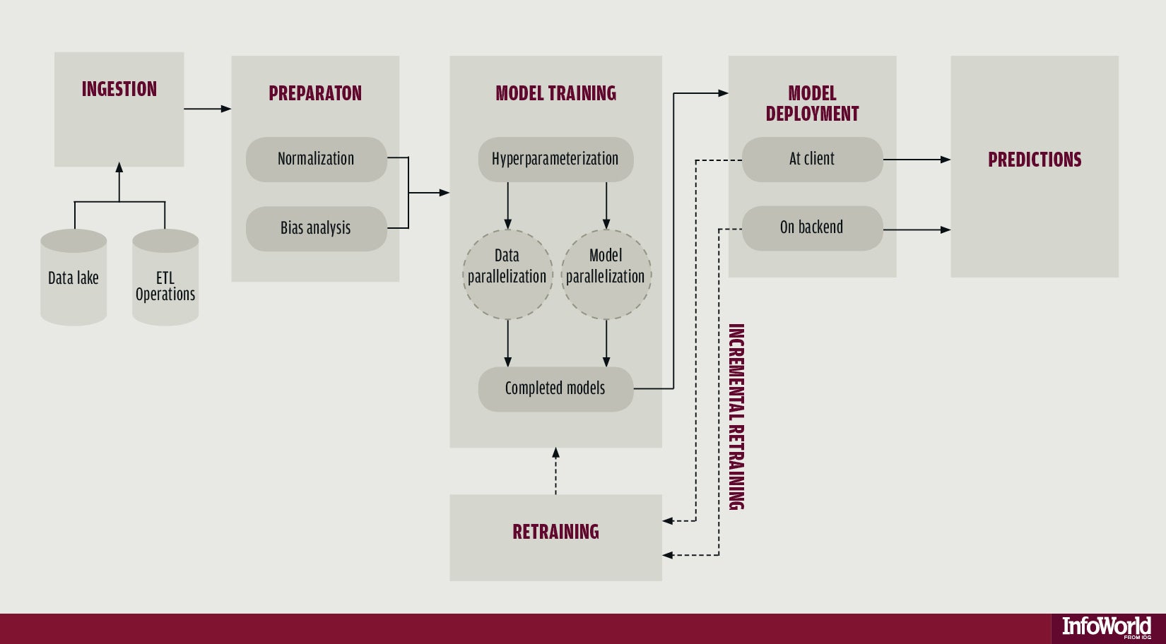
The machine learning pipeline
The four main phases are:
- Data ingestion
- Data preparation / preprocessing
- Models training
- Prediction
12.3.1 Data ingestion
The raw data is loaded. When the data is to big for RAM see ??. It is important that any manipulation on the raw data will be documented, for reproducability, that is, any subsetting, cleaning, arranging will be perform by code. The rational here, is that when new data comes, it will pass through the pipeline without having to do anything manually.
12.3.2 Preparation and Preprocessing
If you use a hold-out set for testing (that’s what I teach here, but testing can be performed repeatedly as in the training-validation CV, by defining inner (train-validation) and outer (train-test) foldings) than splitting is done at the beginning of this stage, before any preprocessing.
After you left some of the data aside for testing, you do all your preprocessing on the remaining.
In the preprocessing step you make the data ready to be trained by algorithms. You want the data to be as informative as possible, i.e., that your features would be most suitable for solving the prediction problem. Actions that are sometimes performed at this stage are data scaling, data imputation, bias corrections, outliers handling, dimensionality reduction, feature engineering and more. (Note: in deep learning, some of these are internal to the learning process, i.e., data representation is learned during the Model training phase.)
Before moving to the training, you need to prepare the test set so it will have the same variables and meaning as the training. For example, if you scaled the training set by subtracting from each variable the mean and dividing by its standard error, than you should apply this also to the test set, but with means and standard errors calculated on the test set.
Sometimes this phase involves Exploratory data analysis and visualization, in order to understand patterns in the data whose recognition may affect prediction success.
12.3.3 Models training
Once you have your data set established, next comes the training process, where the data is used to generate a model from which predictions can be made. You will generally try many different algorithms before finding the one that performs best with your data.
In order to evaluate the performance of some algorithm train it on a training set, and test it on the validation set. compare different algorithms using same train and test.
In this stage you also tune your hyperparameters. A hyperparameter for a machine learning model is a setting that governs how the resulting model is produced from the algorithm. These are parameters that are not learned in the fitting itself. You would learn it manually and systemically: train with different hyperparameters values combinations and test the performance over the validation set. chose the hyperparameters which resulted in the best predictive accuracy.
It is highly recommended to use cross-validation so the results would be more robust.
After convincing yourself which model is best suited and you have tuned the hyperparameters you finally have learner, and you are ready for the next step.
12.3.4 Prediction
In the last phase of the pipeline, you use your trained learner in order to predict with the target in new data. If you saved a test set, you can estimate the performance of this learner with it and report it.
12.4 The caret Package
The caret package (short for Classification And REgression Training) is a set of functions that attempt to streamline the process for creating predictive models. The package contains tools for:
- data splitting
- pre-processing
- feature selection
- model tuning using resampling
- variable importance estimation
as well as other functionality.
There are many different modeling functions in R. Some have different syntax for model training and/or prediction. The package started off as a way to provide a uniform interface the functions themselves, as well as a way to standardize common tasks (such parameter tuning and variable importance).
caret is well documented online. See here, here and here.
12.4.1 Pre-Processing
See caret documentation for more on pre-processing.
12.4.1.1 Zero- and Near Zero-Variance Predictors
Identify variables with very small variance or not at all. There are many models where predictors with a single or almost single unique values (zero- and near zero- variance predictors) will cause the model to fail. We are concerned about this, especially when we split our data into subsamples. Deciding when to Include or not these features is a gentle art (see Kuhn and others (2008)). Anyway, with nearZeroVar() function you would be able to quickly identify these. Type ?nearZeroVar to know exactly how.
##
##   0   1   2
## 501   4  23
nzv <- nearZeroVar(mdrrDescr, saveMetrics= TRUE)
head(nzv[nzv$nzv,]) # get a table of values identified as "Near Zero-Variance Predictors"(nzv$nzv == TRUE) ## freqRatio percentUnique zeroVar nzv
## nTB 23.00000 0.3787879 FALSE TRUE
## nBR 131.00000 0.3787879 FALSE TRUE
## nI 527.00000 0.3787879 FALSE TRUE
## nR03 527.00000 0.3787879 FALSE TRUE
## nR08 527.00000 0.3787879 FALSE TRUE
## nR11 21.78261 0.5681818 FALSE TRUE12.4.2 Centering and Scaling
Centering and Scaling is highly recommended before training, especially from computational perspective. Note that after these transformations you lose the numerical reasoning of the variables’ effects (important only if you are interested in statistical inference)
##   Sepal.Length Sepal.Width Petal.Length Petal.Width Species
## 1          5.1         3.5          1.4         0.2  setosa
## 2          4.9         3.0          1.4         0.2  setosa
## 3          4.7         3.2          1.3         0.2  setosa
## 4          4.6         3.1          1.5         0.2  setosa
## 5          5.0         3.6          1.4         0.2  setosa
## 6          5.4         3.9          1.7         0.4  setosa
train <- iris[1:100,]
test <- iris[101:150,]
(preproc <- preProcess(train, method = c("center","scale"))) # note that factors are not transformed## Created from 100 samples and 5 variables
##
## Pre-processing:
## - centered (4)
## - ignored (1)
## - scaled (4)12.4.3 Model Training and Parameter Tuning
This is the most important and interesting stage in the pipeline, and it is very convenient to do it in caret
caret offers many functionalities for training. We start with an example of a regression prediction problem, where we will try to predict the price of a diamond given features like carat, color, clarity, and diamond’s dimensions. For saving time we take a subset of this data. We also randomly split here our data into training and testing sets.
data(diamonds)
db <- diamonds %>% data.table %>% subset(price < 500)

set.seed(1)
intrain <- sample(1:nrow(db), 0.7*nrow(db))
db_train <- db[intrain,]
db_test <- db[-intrain,]
Before training, let’s check the distribution of the diamonds price over the training set:
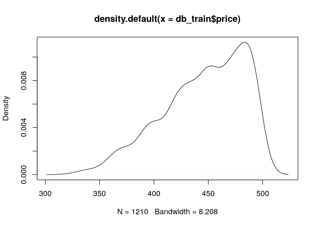
## [1] 445.5512## [1] 37.71684This time, we will use xgboost model for prediction. In caret, Xgboost model’s tunable hyperparameters are max_depth; eta; gamma ; colsample_bytree; min_child_weight and subsample. We will not discuss here the meaning of these parameters (read here if you are interested).
We choose to tune only two hyperparameters: max_depth and eta. The hyperparameters values combinations that we want to consider are defined through the tuneGrid argument in train(). We use expand.grid() to create a data frame from all combinations of the supplied parameters’ values. We look for 4 different max_depth values and 25 different eta values, so this results in 100 different combinations.
tunegrid <- expand.grid(nrounds = 50,
                        max_depth = 2:4,
                        eta = seq(0.05,0.6,length.out = 20),
                        gamma = 0,
                        colsample_bytree = 1,
                        min_child_weight = 1,
                        subsample = 1)
head(tunegrid)
## nrounds max_depth eta gamma colsample_bytree min_child_weight
## 1 50 2 0.05000000 0 1 1
## 2 50 3 0.05000000 0 1 1
## 3 50 4 0.05000000 0 1 1
## 4 50 2 0.07894737 0 1 1
## 5 50 3 0.07894737 0 1 1
## 6 50 4 0.07894737 0 1 1
## subsample
## 1 1
## 2 1
## 3 1
## 4 1
## 5 1
## 6 1The trainControl() function create an object that is passed as the trControl argument in the train() function. This controls the computational nuances of the training. We chose here a 5-fold CV, repeated 3 times. Other built-in cross validation options are: "boot", "cv", "LOOCV", "LGOCV", "repeatedcv", "timeslice", "none" and "oob". We also specify that the parameters’ search approach is a "grid" search (the default). Grid search means that the tuning will be performed by examining every single combination in the grid provided. Other search opportunity is "random" (see here).
Now that we defined the tuning grid and set the training settings, we are ready for the training itself. Note that choosing the set of optimal hyperparameters for a learning algorithm can be a highly computational process, especially for exhaustive searching algorithms such as the grid search. In grid search, the searching time grows exponentially with the number of parameters. Put differently, optimizing p parameters each with k values runs in \(\mathcal{O}(k^p))\) time. Yet, grid search is often embarrassingly parallel.

We combine all these parts together in the train() function. the
# Caution! this might takes few seconds.
xgb_train = caret::train(price ~ .,
                         data=db_train,
                         trControl = trcontrol,
                         tuneGrid = tunegrid,
                         method = "xgbTree")
We can easily plot the tuning results:
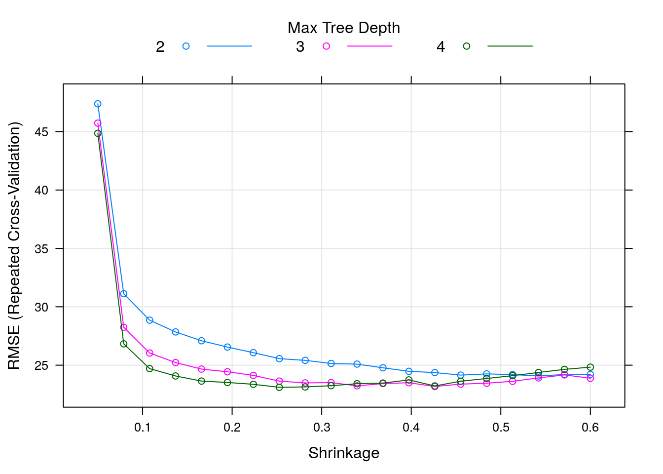
We can see that the RMSE (the lower the better) is in its lowest value when max_depth takes the value of 4, and eta (the shrinkage parameter) is something like 0.25. The optimal combination over the tuneGrid can be obtained by:
##    nrounds max_depth       eta gamma colsample_bytree min_child_weight
## 24      50         4 0.2526316     0                1                1
##    subsample
## 24         1
Let’s check the cross-validated results:
##          eta max_depth gamma colsample_bytree min_child_weight subsample
## 24 0.2526316         4     0                1                1         1
##    nrounds     RMSE  Rsquared      MAE   RMSESD RsquaredSD    MAESD
## 24      50 23.10401 0.6243945 16.51905 1.617463 0.05315021 1.103779
Predicting new dataset is very easy:
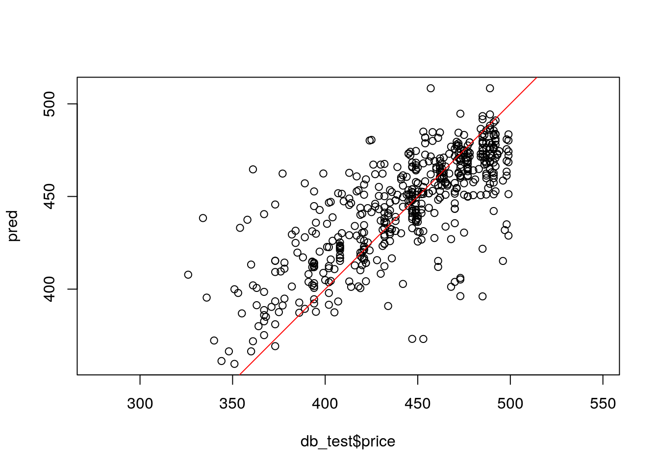
## [1] 25.43778Sometimes it is useful to plot the predictions against the real values to identify any prediction biases.
improve - TODO
Let’s consider another example. This time we will compare different learners in caret. This example is taken from caret tutorial.
This is a problem of classification. We would like to compare 3 different learners:
- Generalized Boosted Tree Model (GBM). Read here about the model
- Support Vector Machines (SVM). Read here
- Regularized Discriminant Analysis (RDA). Good reading here
Our data set We start by splitting to train and test, this time using createDataPartition.
library(mlbench)
data(Sonar)

set.seed(998)
inTraining <- createDataPartition(Sonar$Class, p = .75, list = FALSE)
training <- Sonar[ inTraining,]
testing  <- Sonar[-inTraining,]
We set the training settings:
fitControl <- trainControl(method = "repeatedcv",
                           number = 10,
                           repeats = 10,
                           classProbs = TRUE) ## Estimate class probabilities
The GBM (4 hyperparameters):
gbmGrid <-  expand.grid(interaction.depth = c(1, 5, 9),
                        n.trees = (1:30)*50,
                        shrinkage = 0.1,
                        n.minobsinnode = 20)

gbmFit3 <- train(Class ~ .,
                 data = training,
                 method = "gbm",
                 trControl = fitControl,
                 verbose = FALSE,
                 tuneGrid = gbmGrid)
Let’s have a closer look on the fitted model:
## Stochastic Gradient Boosting
##
## 157 samples
## 60 predictor
## 2 classes: 'M', 'R'
##
## No pre-processing
## Resampling: Cross-Validated (10 fold, repeated 10 times)
## Summary of sample sizes: 142, 141, 141, 140, 142, 141, ...
## Resampling results across tuning parameters:
##
## interaction.depth n.trees Accuracy Kappa
## 1 50 0.7618015 0.5168871
## 1 100 0.7872794 0.5702153
## 1 150 0.8099485 0.6157370
## 1 200 0.8130417 0.6221065
## 1 250 0.8117034 0.6196788
## 1 300 0.8103382 0.6167067
## 1 350 0.8135515 0.6236003
## 1 400 0.8141765 0.6247286
## 1 450 0.8129265 0.6218813
## 1 500 0.8095515 0.6155229
## 1 550 0.8095147 0.6155385
## 1 600 0.8114779 0.6193033
## 1 650 0.8078064 0.6115005
## 1 700 0.8077230 0.6116258
## 1 750 0.8110147 0.6184515
## 1 800 0.8090196 0.6144622
## 1 850 0.8090147 0.6147713
## 1 900 0.8071667 0.6112672
## 1 950 0.8078750 0.6123273
## 1 1000 0.8123333 0.6213103
## 1 1050 0.8123382 0.6214638
## 1 1100 0.8117230 0.6199617
## 1 1150 0.8123015 0.6214193
## 1 1200 0.8103848 0.6174807
## 1 1250 0.8091765 0.6147302
## 1 1300 0.8053382 0.6070300
## 1 1350 0.8079681 0.6123225
## 1 1400 0.8085098 0.6135119
## 1 1450 0.8103480 0.6173126
## 1 1500 0.8127328 0.6220555
## 5 50 0.7852426 0.5656744
## 5 100 0.8071299 0.6108882
## 5 150 0.8162966 0.6287662
## 5 200 0.8206348 0.6374661
## 5 250 0.8224314 0.6405798
## 5 300 0.8276814 0.6515419
## 5 350 0.8295613 0.6555247
## 5 400 0.8268211 0.6502356
## 5 450 0.8254926 0.6475683
## 5 500 0.8294926 0.6553293
## 5 550 0.8313260 0.6593640
## 5 600 0.8285809 0.6534296
## 5 650 0.8299559 0.6564307
## 5 700 0.8299975 0.6565287
## 5 750 0.8281225 0.6528153
## 5 800 0.8275760 0.6517332
## 5 850 0.8299926 0.6563770
## 5 900 0.8299093 0.6565288
## 5 950 0.8299926 0.6563103
## 5 1000 0.8318309 0.6601520
## 5 1050 0.8312843 0.6591066
## 5 1100 0.8313627 0.6591201
## 5 1150 0.8305760 0.6577171
## 5 1200 0.8344510 0.6651799
## 5 1250 0.8332377 0.6628385
## 5 1300 0.8344877 0.6653378
## 5 1350 0.8325760 0.6616264
## 5 1400 0.8333211 0.6630119
## 5 1450 0.8339044 0.6643353
## 5 1500 0.8338676 0.6641615
## 9 50 0.7912230 0.5772602
## 9 100 0.8169436 0.6307056
## 9 150 0.8247696 0.6460877
## 9 200 0.8204877 0.6375483
## 9 250 0.8287377 0.6537923
## 9 300 0.8254926 0.6472631
## 9 350 0.8297525 0.6559470
## 9 400 0.8305025 0.6571102
## 9 450 0.8269044 0.6497061
## 9 500 0.8317157 0.6593368
## 9 550 0.8299142 0.6556403
## 9 600 0.8274828 0.6510078
## 9 650 0.8279093 0.6520596
## 9 700 0.8280809 0.6520968
## 9 750 0.8274559 0.6512011
## 9 800 0.8268260 0.6498980
## 9 850 0.8273775 0.6509871
## 9 900 0.8299608 0.6560862
## 9 950 0.8279191 0.6519843
## 9 1000 0.8304608 0.6569792
## 9 1050 0.8272892 0.6504999
## 9 1100 0.8304191 0.6567004
## 9 1150 0.8303775 0.6564868
## 9 1200 0.8324559 0.6604038
## 9 1250 0.8304608 0.6566592
## 9 1300 0.8323775 0.6608814
## 9 1350 0.8330074 0.6619404
## 9 1400 0.8304706 0.6571329
## 9 1450 0.8311324 0.6585739
## 9 1500 0.8285074 0.6533209
##
## Tuning parameter 'shrinkage' was held constant at a value of 0.1
##
## Tuning parameter 'n.minobsinnode' was held constant at a value of 20
## Accuracy was used to select the optimal model using the largest value.
## The final values used for the model were n.trees = 1300,
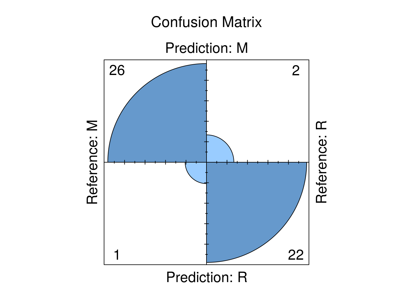
## interaction.depth = 5, shrinkage = 0.1 and n.minobsinnode = 20.Let’s take as look on the confusion Matrix:
## Confusion Matrix and Statistics
##
##           Reference
## Prediction  M  R
##          M 26  2
##          R  1 22
##
##                Accuracy : 0.9412
##                  95% CI : (0.8376, 0.9877)
##     No Information Rate : 0.5294
##     P-Value [Acc > NIR] : 1.285e-10
##
##                   Kappa : 0.8817
##
##  Mcnemar's Test P-Value : 1
##
##             Sensitivity : 0.9630
##             Specificity : 0.9167
##          Pos Pred Value : 0.9286
##          Neg Pred Value : 0.9565
##              Prevalence : 0.5294
##          Detection Rate : 0.5098
##    Detection Prevalence : 0.5490
##       Balanced Accuracy : 0.9398
##
##        'Positive' Class : M
##
We can also nicely plot it:
Now SVM. We ask for centering and scaling as well (very recommended for SVM). This model has only one parameter, so we can specify the total number of parameter combinations that will be evaluated through tuneLength.
svmFit <- train(Class ~ ., data = training,
                 method = "svmRadial",
                 trControl = fitControl,
                 preProc = c("center", "scale"),
                 tuneLength = 8)
svmFit
## Support Vector Machines with Radial Basis Function Kernel
##
## 157 samples
## 60 predictor
## 2 classes: 'M', 'R'
##
## Pre-processing: centered (60), scaled (60)
## Resampling: Cross-Validated (10 fold, repeated 10 times)
## Summary of sample sizes: 142, 141, 142, 142, 141, 141, ...
## Resampling results across tuning parameters:
##
## C Accuracy Kappa
## 0.25 0.7480025 0.4952783
## 0.50 0.8038382 0.6043890
## 1.00 0.8256789 0.6468129
## 2.00 0.8335392 0.6627342
## 4.00 0.8495735 0.6956278
## 8.00 0.8691250 0.7354276
## 16.00 0.8677598 0.7322687
## 32.00 0.8703799 0.7378582
##
## Tuning parameter 'sigma' was held constant at a value of 0.01102444
## Accuracy was used to select the optimal model using the largest value.
## The final values used for the model were sigma = 0.01102444 and C = 32.rdaFit <- train(Class ~ ., data = training,
method = "rda",
trControl = fitControl,
tuneLength = 4)
rdaFit ## Regularized Discriminant Analysis
##
## 157 samples
## 60 predictor
## 2 classes: 'M', 'R'
##
## No pre-processing
## Resampling: Cross-Validated (10 fold, repeated 10 times)
## Summary of sample sizes: 141, 140, 141, 141, 142, 142, ...
## Resampling results across tuning parameters:
##
## gamma lambda Accuracy Kappa
## 0.0000000 0.0000000 0.6603137 0.2907363
## 0.0000000 0.3333333 0.8134559 0.6224215
## 0.0000000 0.6666667 0.8113088 0.6202195
## 0.0000000 1.0000000 0.7774216 0.5528203
## 0.3333333 0.0000000 0.8234755 0.6418976
## 0.3333333 0.3333333 0.8537279 0.7024871
## 0.3333333 0.6666667 0.8488260 0.6918903
## 0.3333333 1.0000000 0.8102525 0.6168901
## 0.6666667 0.0000000 0.8243333 0.6432689
## 0.6666667 0.3333333 0.8276299 0.6490543
## 0.6666667 0.6666667 0.8308162 0.6565586
## 0.6666667 1.0000000 0.7935343 0.5852531
## 1.0000000 0.0000000 0.6691152 0.3363976
## 1.0000000 0.3333333 0.6703652 0.3384976
## 1.0000000 0.6666667 0.6698137 0.3373950
## 1.0000000 1.0000000 0.6691103 0.3358305
##
## Accuracy was used to select the optimal model using the largest value.
## The final values used for the model were gamma = 0.3333333 and lambda
## = 0.3333333.Given these models, can we make statistical statements about their performance differences? To do this, we first collect the resampling results using resamples.
Accuracy and Kappa are the default metrics used to evaluate algorithms on binary and multi-class classification datasets in caret.
Accuracy is the percentage of correctly classifies instances out of all instances. You may want to compare it to a random guess (e.g., 0.25 in 4 classes prediction) when each class has equal representation in the data, or to classes’ prior distributions. Learn more about Accuracy here.
Kappa is like classification accuracy, except that it is normalized at the baseline of random chance on your dataset, hence, more useful measure to use on problems that have an imbalance in the classes. Learn more about Kappa here.
##
## Call:
## resamples.default(x = list(GBM = gbmFit3, SVM = svmFit, RDA = rdaFit))
##
## Models: GBM, SVM, RDA
## Number of resamples: 100
## Performance metrics: Accuracy, Kappa
## Time estimates for: everything, final model fit##
## Call:
## summary.resamples(object = resamps)
##
## Models: GBM, SVM, RDA
## Number of resamples: 100
##
## Accuracy
## Min. 1st Qu. Median Mean 3rd Qu. Max. NA's
## GBM 0.6250 0.8000000 0.8666667 0.8344877 0.8823529 1 0
## SVM 0.5625 0.8207721 0.8750000 0.8703799 0.9343750 1 0
## RDA 0.6250 0.8000000 0.8666667 0.8537279 0.9333333 1 0
##
## Kappa
## Min. 1st Qu. Median Mean 3rd Qu. Max. NA's
## GBM 0.2500000 0.5945946 0.7272727 0.6653378 0.7613948 1 0
## SVM 0.1250000 0.6349734 0.7460317 0.7378582 0.8681844 1 0
## RDA 0.2131148 0.5945946 0.7321429 0.7024871 0.8648649 1 0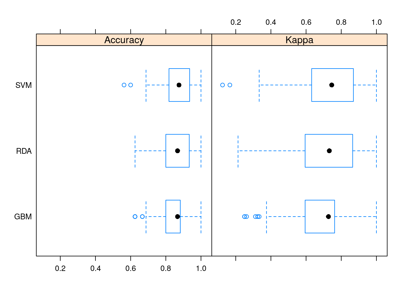
It seems that SVM did a better job of all the learners.
12.5 The mlr Package
Similar to caret, the mlr (short Machine Learning in R) provide a generic and standardized interface for R’s machine learning algorithms with efficient parallelization. That’s include model resampling, hyperparameters optimization, features selection, pre- and post- data-processing, and models comparison.
mlr documentation is also wide (see mlr tutorial, mlr cheat shhet, )
mlr has some advantages over caret especially in:
- Providing more parallelization possibilities.
- Providing more possibilities for creating different tasks.
- Tuning: using the mlrMBO Bayesian optimization package. It is HIGHLY recommended to be familiar with this package.
We will not cover the mlr package in this course, but students are encouraged to experience it themselves.
12.6 Bibliographic Notes
TODO
12.7 Practice Yourself
TODO
References
Kuhn, Max, and others. 2008. “Building Predictive Models in R Using the Caret Package.” Journal of Statistical Software 28 (5): 1–26.