Chapter 8 Generalized Linear Models

Example 8.1 Consider the relation between cigarettes smoked, and the occurance of lung cancer. Do we expect the probability of cancer to be linear in the number of cigarettes? Probably not. Do we expect the variability of events to be constant about the trend? Probably not.

Example 8.2 Consider the relation between the travel times to the distance travelled. Do you agree that the longer the distance travelled, then not only the travel times get longer, but they also get more variable?

8.1 Problem Setup

In the Linear Models Chapter 7, we assumed the generative process to be linear in the effects of the predictors \(x\). We now write that same linear model, slightly differently: \[ y|x \sim \mathcal{N}(x'\beta, \sigma^2). \]

This model not allow for the non-linear relations of Example 8.1, nor does it allow for the distrbituion of \(\varepsilon\) to change with \(x\), as in Example 8.2. Generalize linear models (GLM), as the name suggests, are a generalization of the linear models in Chapter 7 that allow that¹³.

For Example 8.1, we would like something in the lines of \[ y|x \sim Binom(1,p(x)) \]

For Example 8.2, we would like something in the lines of \[ y|x \sim \mathcal{N}(x'\beta,\sigma^2(x)), \] or more generally \[ y|x \sim \mathcal{N}(\mu(x),\sigma^2(x)), \] or maybe not Gaussian \[ y|x \sim Pois(\lambda(x)). \]

Even more generally, for some distribution \(F(\theta)\), with a parameter \(\theta\), we would like to assume that the data is generated via \[\begin{align} \tag{8.1} y|x \sim F(\theta(x)) \end{align}\]

Possible examples include \[\begin{align} y|x &\sim Poisson(\lambda(x)) \\ y|x &\sim Exp(\lambda(x)) \\ y|x &\sim \mathcal{N}(\mu(x),\sigma^2(x)) \end{align}\]

GLMs allow models of the type of Eq.(8.1), while imposing some constraints on \(F\) and on the relation \(\theta(x)\). GLMs assume the data distribution \(F\) to be in a “well-behaved” family known as the Natural Exponential Family of distributions. This family includes the Gaussian, Gamma, Binomial, Poisson, and Negative Binomial distributions. These five include as special cases the exponential, chi-squared, Rayleigh, Weibull, Bernoulli, and geometric distributions.

GLMs also assume that the distribution’s parameter, \(\theta\), is some simple function of a linear combination of the effects. In our cigarettes example this amounts to assuming that each cigarette has an additive effect, but not on the probability of cancer, but rather, on some simple function of it. Formally \[g(\theta(x))=x'\beta,\] and we recall that \[x'\beta=\beta_0 + \sum_j x_j \beta_j.\] The linear predictor \(x'\beta\) is usually denoted by \(\eta\), i.e., \(\eta = x'\beta\) The function \(g\) is called the link function, its inverse, \(g^{-1}\) is the mean function. It is called the mean function as \[E(y|x) = \mu = g^{-1}(\eta)\].

We say that “the effects of each cigarette is linear in link scale”. This terminology will later be required to understand R’s output.

8.2 Logistic Regression

The best known of the GLM class of models is the logistic regression that deals with Binomial, or more precisely, Bernoulli-distributed data. The link function in the logistic regression is the logit function \[\begin{align} g(t)=log\left( \frac{t}{(1-t)} \right) \tag{8.2} \end{align}\] implying that under the logistic model assumptions \[\begin{align} y|x \sim Binom \left( 1, p=\frac{e^{x'\beta}}{1+e^{x'\beta}} \right). \tag{8.3} \end{align}\]

Before we fit such a model, we try to justify this construction, in particular, the enigmatic link function in Eq.(8.2). Let’s look at the simplest possible case: the comparison of two groups indexed by \(x\): \(x=0\) for the first, and \(x=1\) for the second. We start with some definitions.

Definition 8.1 (Odds) The odds, of a binary random variable, \(y\), is defined as \[\frac{P(y=1)}{P(y=0)}.\]

Odds are the same as probabilities, but instead of telling me there is a \(66\%\) of success, they tell me the odds of success are “2 to 1”. If you ever placed a bet, the language of “odds” should not be unfamiliar to you.

Definition 8.2 (Odds Ratio) The odds ratio between two binary random variables, \(y_1\) and \(y_2\), is defined as the ratio between their odds. Formally: \[OR(y_1,y_2):=\frac{P(y_1=1)/P(y_1=0)}{P(y_2=1)/P(y_2=0)}.\]

Odds ratios (OR) compare between the probabilities of two groups, only that it does not compare them in probability scale, but rather in odds scale. You can also think of ORs as a measure of distance between two Brenoulli distributions. ORs have better mathematical properties than other candidate distance measures, such as \(P(y_1=1)-P(y_2=1)\).

Under the logit link assumption formalized in Eq.(8.3), the OR between two conditions indexed by \(y|x=1\) and \(y|x=0\), returns: \[\begin{align} OR(y|x=1,y|x=0) = \frac{P(y=1|x=1)/P(y=0|x=1)}{P(y=1|x=0)/P(y=0|x=0)} = e^{\beta_1}. \end{align}\]

The last equality demystifies the choice of the link function in the logistic regression: it allows us to interpret \(\beta\) of the logistic regression as a measure of change of binary random variables, namely, as the (log) odds-ratios due to a unit increase in \(x\).

Remark. Another popular link function is the normal quantile function, a.k.a., the Gaussian inverse CDF, leading to probit regression instead of logistic regression.

8.2.1 Logistic Regression with R

Let’s get us some data. The PlantGrowth data records the weight of plants under three conditions: control, treatment1, and treatment2.

head(PlantGrowth)

##   weight group
## 1   4.17  ctrl
## 2   5.58  ctrl
## 3   5.18  ctrl
## 4   6.11  ctrl
## 5   4.50  ctrl
## 6   4.61  ctrl

We will now attach the data so that its contents is available in the workspace (don’t forget to detach afterwards, or you can expect some conflicting object names). We will also use the cut function to create a binary response variable for Light, and Heavy plants (we are doing logistic regression, so we need a two-class response). As a general rule of thumb, when we discretize continuous variables, we lose information. For pedagogical reasons, however, we will proceed with this bad practice.

Look at the following output and think: how many group effects do we expect? What should be the sign of each effect?

attach(PlantGrowth)
weight.factor<- cut(weight, 2, labels=c('Light', 'Heavy')) # binarize weights
plot(table(group, weight.factor))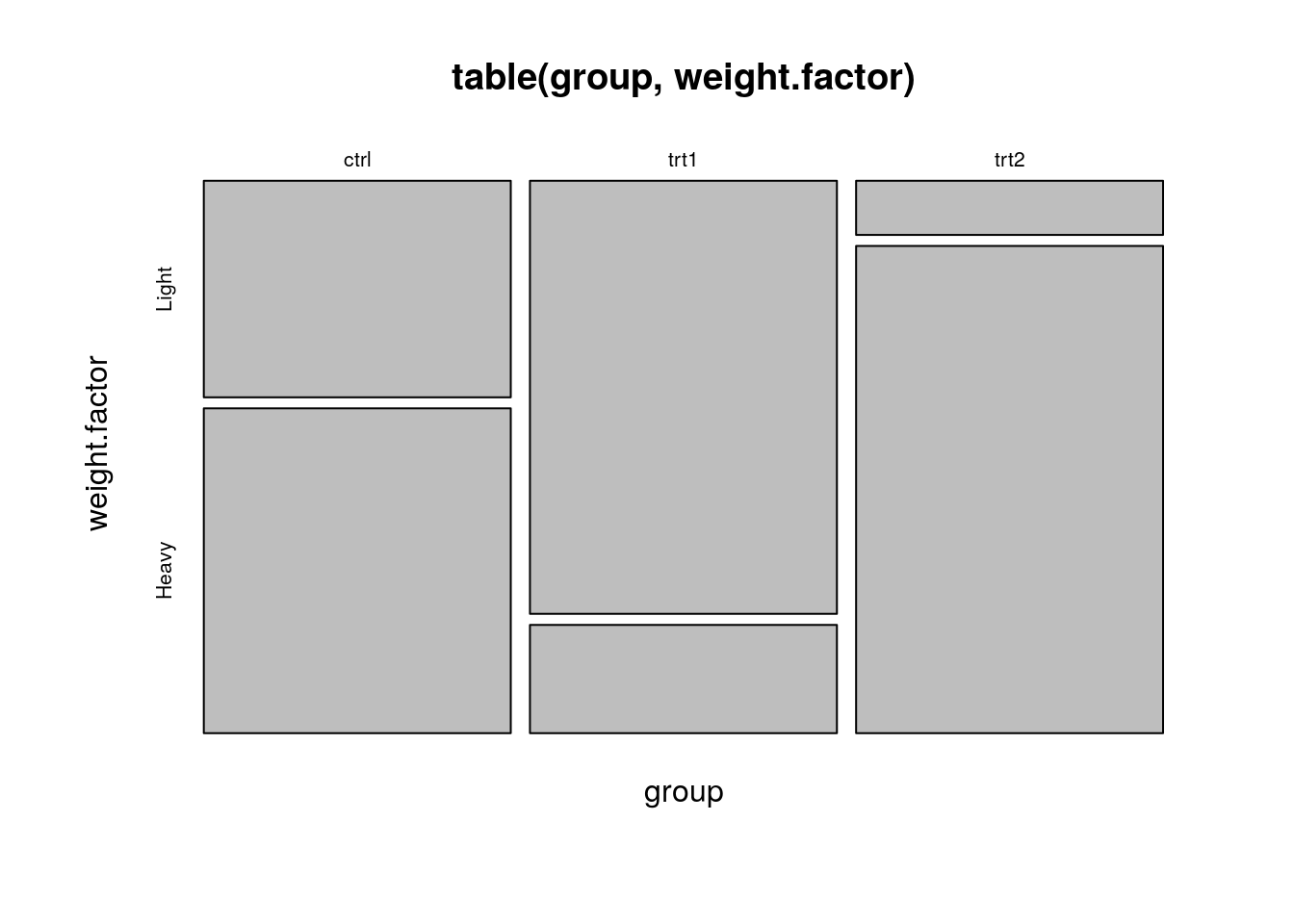

Let’s fit a logistic regression, and inspect the output.

glm.1<- glm(weight.factor~group, family=binomial)
summary(glm.1)

## 
## Call:
## glm(formula = weight.factor ~ group, family = binomial)
## 
## Deviance Residuals: 
##     Min       1Q   Median       3Q      Max  
## -2.1460  -0.6681   0.4590   0.8728   1.7941  
## 
## Coefficients:
##             Estimate Std. Error z value Pr(>|z|)  
## (Intercept)   0.4055     0.6455   0.628   0.5299  
## grouptrt1    -1.7918     1.0206  -1.756   0.0792 .
## grouptrt2     1.7918     1.2360   1.450   0.1471  
## ---
## Signif. codes:  0 '***' 0.001 '**' 0.01 '*' 0.05 '.' 0.1 ' ' 1
## 
## (Dispersion parameter for binomial family taken to be 1)
## 
##     Null deviance: 41.054  on 29  degrees of freedom
## Residual deviance: 29.970  on 27  degrees of freedom
## AIC: 35.97
## 
## Number of Fisher Scoring iterations: 4

Things to note:

• The glm function is our workhorse for all GLM models.

• The family argument of glm tells R the respose variable is brenoulli, thus, performing a logistic regression.

• The summary function is content aware. It gives a different output for glm class objects than for other objects, such as the lm we saw in Chapter 7. In fact, what summary does is merely call summary.glm.

• As usual, we get the coefficients table, but recall that they are to be interpreted as (log) odd-ratios, i.e., in “link scale”. To return to probabilities (“response scale”), we will need to undo the logistic transformation.

• As usual, we get the significance for the test of no-effect, versus a two-sided alternative. P-values are asymptotic, thus, only approximate (and can be very bad approximations in small samples).

• The residuals of glm are slightly different than the lm residuals, and called Deviance Residuals.

• AIC (Akaike Information Criteria) is the equivalent of R2 in logistic regression. It measures the fit when a penalty is applied to the number of parameters (see AIC definition here). Smaller AIC values indicate the model is closer to the truth.

• Null deviance: Fits the model only with the intercept. The degree of freedom is n-1. We can interpret it as a Chi-square value (fitted value different from the actual value hypothesis testing).

• Residual Deviance: Model with all the variables. It is also interpreted as a Chi-square hypothesis testing.

• Number of Fisher Scoring iterations: Number of iterations before converging ().

• For help see ?glm, ?family, and ?summary.glm.

Like in the linear models, we can use an ANOVA table to check if treatments have any effect, and not one treatment at a time. In the case of GLMs, this is called an analysis of deviance table.

anova(glm.1, test='LRT')

## Analysis of Deviance Table
## 
## Model: binomial, link: logit
## 
## Response: weight.factor
## 
## Terms added sequentially (first to last)
## 
## 
##       Df Deviance Resid. Df Resid. Dev Pr(>Chi)   
## NULL                     29     41.054            
## group  2   11.084        27     29.970 0.003919 **
## ---
## Signif. codes:  0 '***' 0.001 '**' 0.01 '*' 0.05 '.' 0.1 ' ' 1

Things to note:

• The anova function, like the summary function, are content-aware and produce a different output for the glm class than for the lm class. All that anova does is call anova.glm.
• In GLMs there is no canonical test (like the F test for lm). LRT implies we want an approximate Likelihood Ratio Test. We thus specify the type of test desired with the test argument.
• The distribution of the weights of the plants does vary with the treatment given, as we may see from the significance of the group factor.
• Readers familiar with ANOVA tables, should know that we computed the GLM equivalent of a type I sum- of-squares. Run drop1(glm.1, test='Chisq') for a GLM equivalent of a type III sum-of-squares.
• For help see ?anova.glm.

Let’s predict the probability of a heavy plant for each treatment.

predict(glm.1, type='response')

##   1   2   3   4   5   6   7   8   9  10  11  12  13  14  15  16  17  18 
## 0.6 0.6 0.6 0.6 0.6 0.6 0.6 0.6 0.6 0.6 0.2 0.2 0.2 0.2 0.2 0.2 0.2 0.2 
##  19  20  21  22  23  24  25  26  27  28  29  30 
## 0.2 0.2 0.9 0.9 0.9 0.9 0.9 0.9 0.9 0.9 0.9 0.9

Things to note:

• Like the summary and anova functions, the predict function is aware that its input is of glm class. All that predict does is call predict.glm.
• In GLMs there are many types of predictions. The type argument controls which type is returned. Use type=response for predictions in probability scale; use `type=link’ for predictions in log-odds scale.
• How do I know we are predicting the probability of a heavy plant, and not a light plant? Just run contrasts(weight.factor) to see which of the categories of the factor weight.factor is encoded as 1, and which as 0.
• For help see ?predict.glm.

Let’s detach the data so it is no longer in our workspace, and object names do not collide.

detach(PlantGrowth)

We gave an example with a factorial (i.e. discrete) predictor. We can do the same with multiple continuous predictors.

data('Pima.te', package='MASS') # Loads data
head(Pima.te)

##   npreg glu bp skin  bmi   ped age type
## 1     6 148 72   35 33.6 0.627  50  Yes
## 2     1  85 66   29 26.6 0.351  31   No
## 3     1  89 66   23 28.1 0.167  21   No
## 4     3  78 50   32 31.0 0.248  26  Yes
## 5     2 197 70   45 30.5 0.158  53  Yes
## 6     5 166 72   19 25.8 0.587  51  Yes

glm.2<- step(glm(type~., data=Pima.te, family=binomial))

## Start:  AIC=301.79
## type ~ npreg + glu + bp + skin + bmi + ped + age
## 
##         Df Deviance    AIC
## - skin   1   286.22 300.22
## - bp     1   286.26 300.26
## - age    1   286.76 300.76
## <none>       285.79 301.79
## - npreg  1   291.60 305.60
## - ped    1   292.15 306.15
## - bmi    1   293.83 307.83
## - glu    1   343.68 357.68
## 
## Step:  AIC=300.22
## type ~ npreg + glu + bp + bmi + ped + age
## 
##         Df Deviance    AIC
## - bp     1   286.73 298.73
## - age    1   287.23 299.23
## <none>       286.22 300.22
## - npreg  1   292.35 304.35
## - ped    1   292.70 304.70
## - bmi    1   302.55 314.55
## - glu    1   344.60 356.60
## 
## Step:  AIC=298.73
## type ~ npreg + glu + bmi + ped + age
## 
##         Df Deviance    AIC
## - age    1   287.44 297.44
## <none>       286.73 298.73
## - npreg  1   293.00 303.00
## - ped    1   293.35 303.35
## - bmi    1   303.27 313.27
## - glu    1   344.67 354.67
## 
## Step:  AIC=297.44
## type ~ npreg + glu + bmi + ped
## 
##         Df Deviance    AIC
## <none>       287.44 297.44
## - ped    1   294.54 302.54
## - bmi    1   303.72 311.72
## - npreg  1   304.01 312.01
## - glu    1   349.80 357.80

summary(glm.2)

## 
## Call:
## glm(formula = type ~ npreg + glu + bmi + ped, family = binomial, 
##     data = Pima.te)
## 
## Deviance Residuals: 
##     Min       1Q   Median       3Q      Max  
## -2.9845  -0.6462  -0.3661   0.5977   2.5304  
## 
## Coefficients:
##              Estimate Std. Error z value Pr(>|z|)    
## (Intercept) -9.552177   1.096207  -8.714  < 2e-16 ***
## npreg        0.178066   0.045343   3.927  8.6e-05 ***
## glu          0.037971   0.005442   6.978  3.0e-12 ***
## bmi          0.084107   0.021950   3.832 0.000127 ***
## ped          1.165658   0.444054   2.625 0.008664 ** 
## ---
## Signif. codes:  0 '***' 0.001 '**' 0.01 '*' 0.05 '.' 0.1 ' ' 1
## 
## (Dispersion parameter for binomial family taken to be 1)
## 
##     Null deviance: 420.30  on 331  degrees of freedom
## Residual deviance: 287.44  on 327  degrees of freedom
## AIC: 297.44
## 
## Number of Fisher Scoring iterations: 5

Things to note:

• We used the ~. syntax to tell R to fit a model with all the available predictors.
• Since we want to focus on significant predictors, we used the step function to perform a step-wise regression, i.e. sequentially remove non-significant predictors. The function reports each model it has checked, and the variable it has decided to remove at each step.
• The output of step is a single model, with the subset of selected predictors.

8.2.2 Another Logistic regression example and model evaluation

Let’s model the relationship between the probability that an iris flower is of type “setosa”, and the length of its Sepal.

d <- iris
d$is_setosa <- (d$Species=="setosa") * 1

head(d)

##   Sepal.Length Sepal.Width Petal.Length Petal.Width Species is_setosa
## 1          5.1         3.5          1.4         0.2  setosa         1
## 2          4.9         3.0          1.4         0.2  setosa         1
## 3          4.7         3.2          1.3         0.2  setosa         1
## 4          4.6         3.1          1.5         0.2  setosa         1
## 5          5.0         3.6          1.4         0.2  setosa         1
## 6          5.4         3.9          1.7         0.4  setosa         1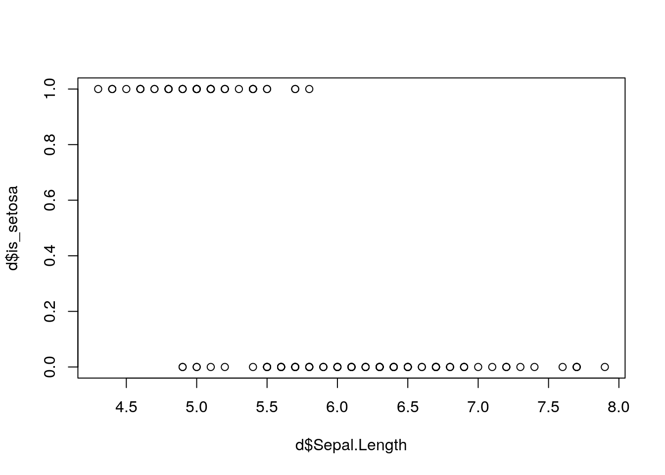

plot(d$is_setosa~d$Sepal.Length)

Again, we do logistic regression. Let’s check the fitted probabilities:

m_glm <- glm(d$is_setosa~d$Sepal.Length, family = binomial)
yhat_glm <- predict(m_glm, type = "response")
hist(yhat_glm)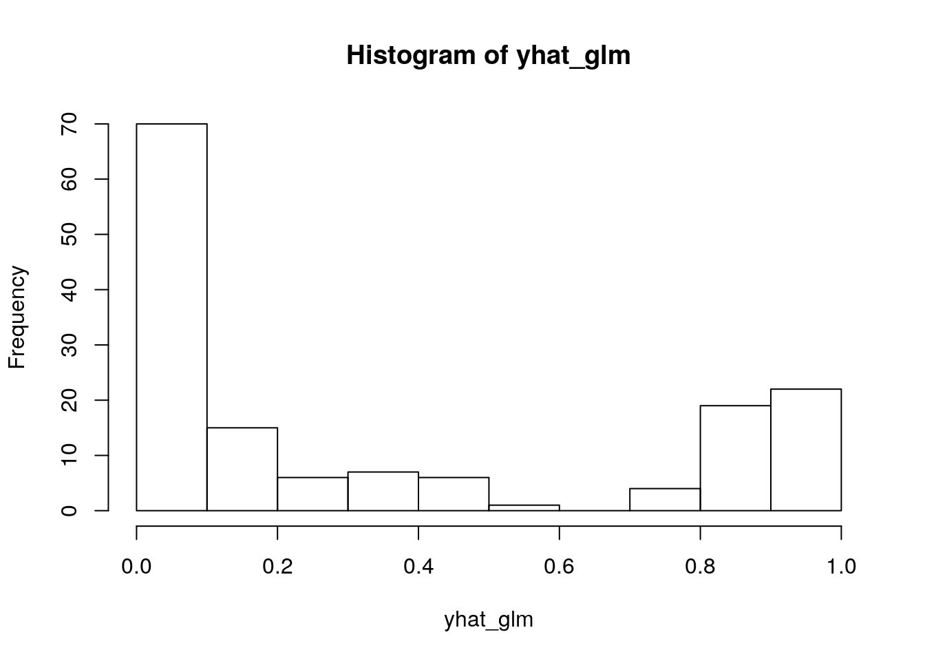

If we are interested in a prediction whether a flower is “setosa” or not, we need a decision rule. A trivial rule is: classify as “1” (’is_setosa`=1) if \(\hat{P}(\text{is_setosa}=1|\text{Sepal.Length})>0.5\)

yhat_glm_binar <- ifelse(yhat_glm>0.5, 1, 0)

We can plot the data and distinguish between samples we classed to 1 and 0. We also add the predicted probabilities and the 0.5 threshold:

plot(d$is_setosa~d$Sepal.Length, col = as.factor(yhat_glm_binar))
lines(yhat_glm[order(d$Sepal.Length)]~d$Sepal.Length[order(d$Sepal.Length)])
abline(h=0.5, lty = 2)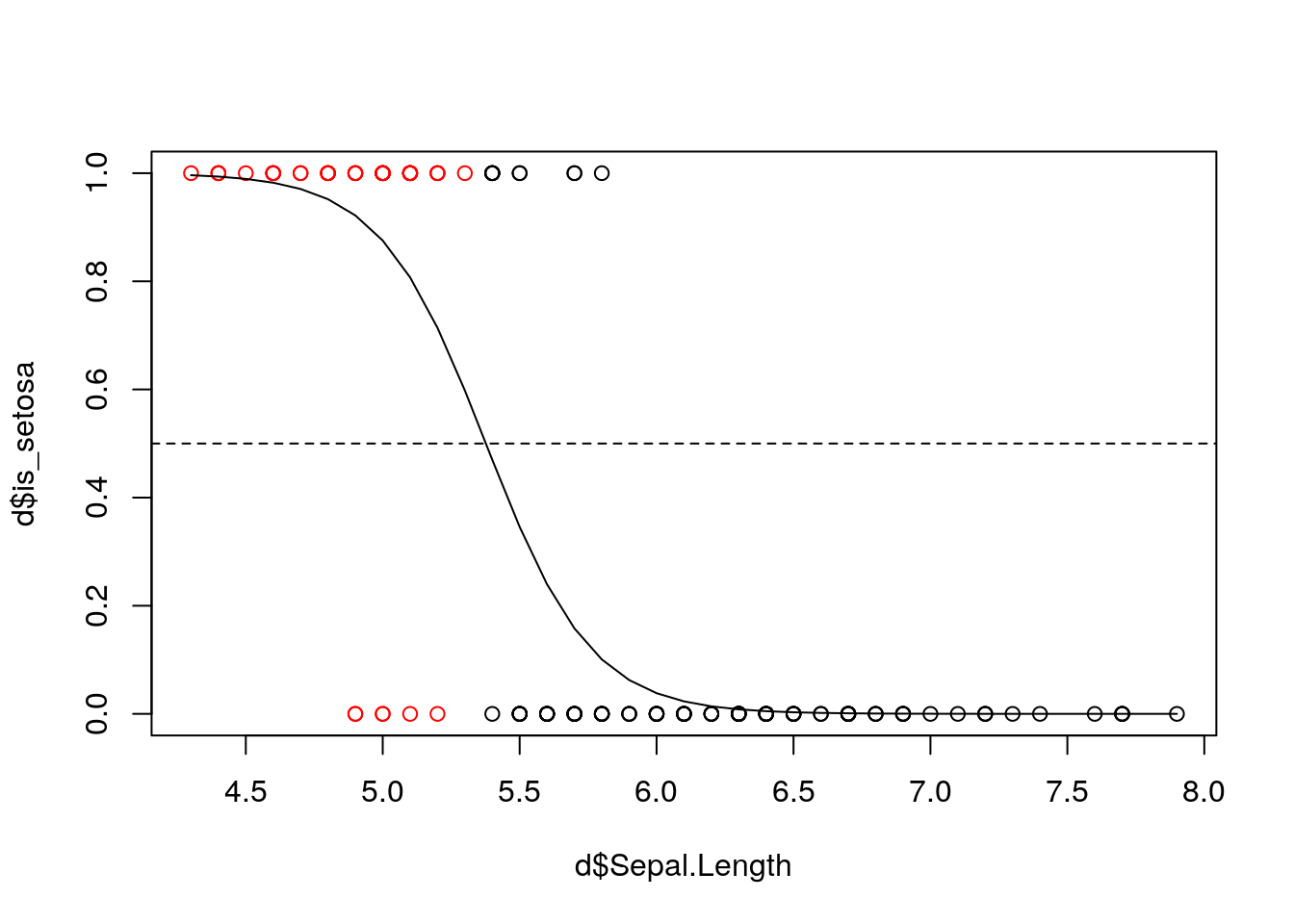

Note that other thresholds are also possible (this is a question of False positives and false negatives)

Let’s compare a logistic and a linear models in a prediction problem. We use the spam dataset from the ElemStatLearn package (see ?ElemStatLearn::spam):

library(ElemStatLearn)
db <- ElemStatLearn::spam
head(db)

##    A.1  A.2  A.3 A.4  A.5  A.6  A.7  A.8  A.9 A.10 A.11 A.12 A.13 A.14
## 1 0.00 0.64 0.64   0 0.32 0.00 0.00 0.00 0.00 0.00 0.00 0.64 0.00 0.00
## 2 0.21 0.28 0.50   0 0.14 0.28 0.21 0.07 0.00 0.94 0.21 0.79 0.65 0.21
## 3 0.06 0.00 0.71   0 1.23 0.19 0.19 0.12 0.64 0.25 0.38 0.45 0.12 0.00
## 4 0.00 0.00 0.00   0 0.63 0.00 0.31 0.63 0.31 0.63 0.31 0.31 0.31 0.00
## 5 0.00 0.00 0.00   0 0.63 0.00 0.31 0.63 0.31 0.63 0.31 0.31 0.31 0.00
## 6 0.00 0.00 0.00   0 1.85 0.00 0.00 1.85 0.00 0.00 0.00 0.00 0.00 0.00
##   A.15 A.16 A.17 A.18 A.19 A.20 A.21 A.22 A.23 A.24 A.25 A.26 A.27 A.28
## 1 0.00 0.32 0.00 1.29 1.93 0.00 0.96    0 0.00 0.00    0    0    0    0
## 2 0.14 0.14 0.07 0.28 3.47 0.00 1.59    0 0.43 0.43    0    0    0    0
## 3 1.75 0.06 0.06 1.03 1.36 0.32 0.51    0 1.16 0.06    0    0    0    0
## 4 0.00 0.31 0.00 0.00 3.18 0.00 0.31    0 0.00 0.00    0    0    0    0
## 5 0.00 0.31 0.00 0.00 3.18 0.00 0.31    0 0.00 0.00    0    0    0    0
## 6 0.00 0.00 0.00 0.00 0.00 0.00 0.00    0 0.00 0.00    0    0    0    0
##   A.29 A.30 A.31 A.32 A.33 A.34 A.35 A.36 A.37 A.38 A.39 A.40 A.41 A.42
## 1    0    0    0    0    0    0    0    0 0.00    0    0 0.00    0    0
## 2    0    0    0    0    0    0    0    0 0.07    0    0 0.00    0    0
## 3    0    0    0    0    0    0    0    0 0.00    0    0 0.06    0    0
## 4    0    0    0    0    0    0    0    0 0.00    0    0 0.00    0    0
## 5    0    0    0    0    0    0    0    0 0.00    0    0 0.00    0    0
## 6    0    0    0    0    0    0    0    0 0.00    0    0 0.00    0    0
##   A.43 A.44 A.45 A.46 A.47 A.48 A.49  A.50 A.51  A.52  A.53  A.54  A.55
## 1 0.00    0 0.00 0.00    0    0 0.00 0.000    0 0.778 0.000 0.000 3.756
## 2 0.00    0 0.00 0.00    0    0 0.00 0.132    0 0.372 0.180 0.048 5.114
## 3 0.12    0 0.06 0.06    0    0 0.01 0.143    0 0.276 0.184 0.010 9.821
## 4 0.00    0 0.00 0.00    0    0 0.00 0.137    0 0.137 0.000 0.000 3.537
## 5 0.00    0 0.00 0.00    0    0 0.00 0.135    0 0.135 0.000 0.000 3.537
## 6 0.00    0 0.00 0.00    0    0 0.00 0.223    0 0.000 0.000 0.000 3.000
##   A.56 A.57 spam
## 1   61  278 spam
## 2  101 1028 spam
## 3  485 2259 spam
## 4   40  191 spam
## 5   40  191 spam
## 6   15   54 spam

db$spam <- 1*(db$spam=="spam")
table(db$spam)

## 
##    0    1 
## 2788 1813

Creating a training and test sets:

set.seed(256)
in_train <- sample(1:nrow(db), 0.5*nrow(db))
db_train <- db[in_train, ]
db_test <- db[-in_train, ]

table(db_train$spam)

## 
##    0    1 
## 1396  904

table(db_test$spam)

## 
##    0    1 
## 1392  909

Comparing the prediction accuracy of the models over a “fresh” test set:

m_lm <- lm(spam ~ ., db_train)
m_glm <- glm(spam ~  ., db_train, family = binomial)

## Warning: glm.fit: fitted probabilities numerically 0 or 1 occurred

y_hat_lm <- predict(m_lm, db_test)
y_hat_glm <- predict(m_glm, db_test, type = "response")

y_hat_lm_binar <- (y_hat_lm>0.5)*1
y_hat_glm_binar <- (y_hat_glm>0.5)*1


mean(db_test$spam==y_hat_lm_binar)

## [1] 0.8813559

mean(db_test$spam==y_hat_glm_binar)

## [1] 0.9269883

It seems that the logistic regression does a better job

8.2.3 Measuring Accuracy, Precision and Recall:

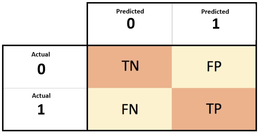
Confusion Matrix

In the field of machine learning and specifically the problem of statistical classification, a confusion matrix, also known as an error matrix, is a specific table layout that allows visualization of the performance of a prediction algorithm (as logistic regression), typically a supervised learning one. Each row of the matrix represents the instances in a predicted class while each column represents the instances in an actual class (or vice versa). The name stems from the fact that it makes it easy to see if the system is confusing two classes (i.e. commonly mislabeling one as another).

The confusion matrix is a better choice to evaluate the classification performance compared with the different metrics as AIC which you saw before - it compute the performance on new set, which we did not use at model fitting. The general idea is to count the number of times True/False instances are classified as True/False:

confusion matrix

It can be obtained by:

(CM <- table(true= db_test$spam, predicted = y_hat_glm_binar))

##     predicted
## true    0    1
##    0 1330   62
##    1  106  803

The Accuracy is defined as: \[Accuracy = \frac{TP + TN}{TP + TN + FP + FN}\] and can be obtained with:

sum(diag(CM)) / sum(CM)

## [1] 0.9269883

But accuracy can sometimes be a bad metric for predictive classification models (see The Accuracy Paradox. For example, if the incidence of category A is dominant, being found in 99% of cases, then predicting that every case is category A will have an accuracy of 99%. In that case an unuseful model may have a high level of accuracy.

Precision and recall are better measures in such cases. \[Precision = \frac{TP}{TP + FP}\] \[Recall = \frac{TP}{TP + FN}\] Precision looks at the accuracy of the positive prediction. Recall is the ratio of positive instances that are correctly detected by the classifier. While recall expresses the ability to find all relevant instances in a dataset, precision expresses the proportion of the data points our model says was relevant actually were relevant.

We can get them with:

(Precision <- CM[4] / sum(CM[,2]))

## [1] 0.9283237

(Recall <- CM[4] / sum(CM[2,]))

## [1] 0.8833883

Note that we can not have have high precision and high recall at the same time, and there is a tradeoff between the two. Precision is more important than Recall when you would like to have less False Positives in trade off to have more False Negatives. Meaning, getting a False Positive is very costly, and a False Negative is not as much. In some situations, we might know that we want to maximize either recall or precision at the expense of the other metric. For example, in preliminary disease screening of patients for follow-up examinations, we would probably want a recall near 1.0, as we want to find all patients who actually have the disease, and we can accept a low precision if the cost of the follow-up examination is not significant. You may know this tradoff as Type I and type II errors in statistical hypothesis testing.

In cases where we want to find an optimal blend of precision and recall we can combine the two metrics using what is called the F1 score: \[ F_1 = 2 \frac{precision*recall}{precision+recall}\].

There is a concave relationship between precision and recall. The ROC curve is a graphical plot that illustrates the diagnostic ability of a binary classification model (such as the logistic regression) as its discrimination threshold is varied. The ROC curve is created by plotting the True Positive Rate (Recall) against the False Positive Rate (\(FP/(FP+TN)\)) at various threshold settings.

here is an example of how to compute it:

alphas <- seq(0,1,0.01)
TPRs <- numeric(length(alphas))
FPRs <- numeric(length(alphas))
for (i in seq_along(alphas)) {
  pr_i <- ifelse(y_hat_glm>alphas[i],1,0)
  CM_i <- table(db_test$spam, pr_i)
  TPRs[i] <- CM_i[4] / sum(CM_i[2,])
  FPRs[i] <- CM_i[3] / sum(CM_i[1,])
}
plot(TPRs~FPRs, type = "l")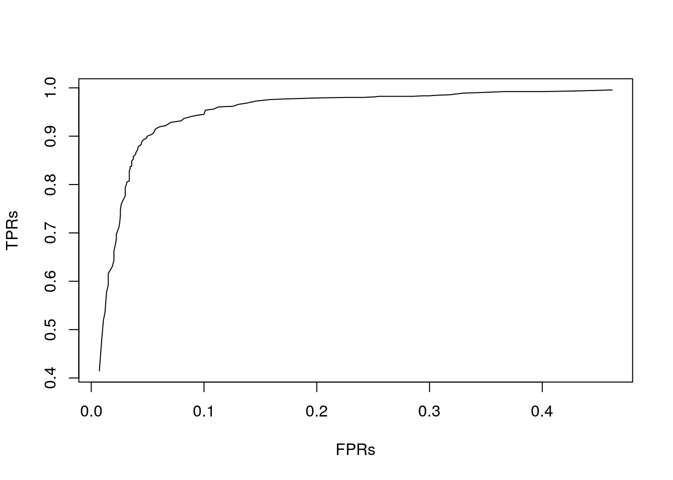

And see here fancier ROC libraries, e.g., with the ROCit package:

library("ROCit")
ROCit_obj <- rocit(score=y_hat_glm,class=db_test$spam)
plot(ROCit_obj)

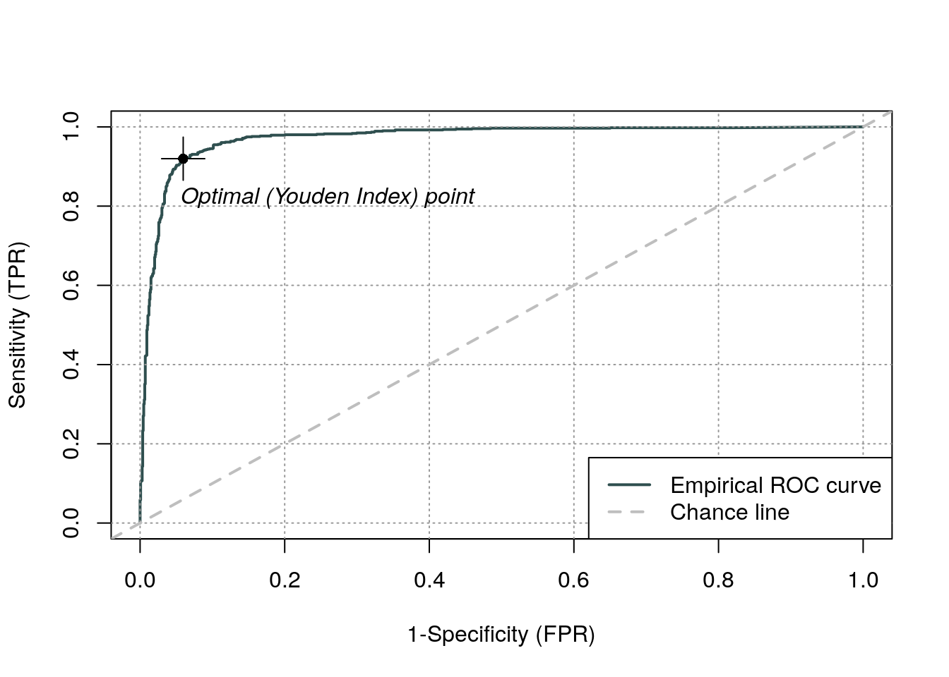
ROC analysis provides tools to select possibly optimal models and to discard suboptimal ones independently from (and prior to specifying) the cost context or the class distribution.

The ROC space for a “better” and “worse” classfier. Source: Wikipedia

8.3 Poisson Regression

Poisson regression means we fit a model assuming \(y|x \sim Poisson(\lambda(x))\). Put differently, we assume that for each treatment, encoded as a combinations of predictors \(x\), the response is Poisson distributed with a rate that depends on the predictors.

The typical link function for Poisson regression is the logarithm: \(g(t)=log(t)\). This means that we assume \(y|x \sim Poisson(\lambda(x) = e^{x'\beta})\). Why is this a good choice? We again resort to the two-group case, encoded by \(x=1\) and \(x=0\), to understand this model: \(\lambda(x=1)=e^{\beta_0+\beta_1}=e^{\beta_0} \; e^{\beta_1}= \lambda(x=0) \; e^{\beta_1}\). We thus see that this link function implies that a change in \(x\) multiples the rate of events by \(e^{\beta_1}\).

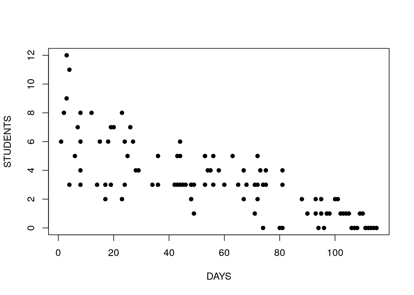
For our example¹⁴ we inspect the number of infected high-school kids, as a function of the days since an outbreak.

cases <-  
structure(list(Days = c(1L, 2L, 3L, 3L, 4L, 4L, 4L, 6L, 7L, 8L, 
8L, 8L, 8L, 12L, 14L, 15L, 17L, 17L, 17L, 18L, 19L, 19L, 20L, 
23L, 23L, 23L, 24L, 24L, 25L, 26L, 27L, 28L, 29L, 34L, 36L, 36L, 
42L, 42L, 43L, 43L, 44L, 44L, 44L, 44L, 45L, 46L, 48L, 48L, 49L, 
49L, 53L, 53L, 53L, 54L, 55L, 56L, 56L, 58L, 60L, 63L, 65L, 67L, 
67L, 68L, 71L, 71L, 72L, 72L, 72L, 73L, 74L, 74L, 74L, 75L, 75L, 
80L, 81L, 81L, 81L, 81L, 88L, 88L, 90L, 93L, 93L, 94L, 95L, 95L, 
95L, 96L, 96L, 97L, 98L, 100L, 101L, 102L, 103L, 104L, 105L, 
106L, 107L, 108L, 109L, 110L, 111L, 112L, 113L, 114L, 115L), 
    Students = c(6L, 8L, 12L, 9L, 3L, 3L, 11L, 5L, 7L, 3L, 8L, 
    4L, 6L, 8L, 3L, 6L, 3L, 2L, 2L, 6L, 3L, 7L, 7L, 2L, 2L, 8L, 
    3L, 6L, 5L, 7L, 6L, 4L, 4L, 3L, 3L, 5L, 3L, 3L, 3L, 5L, 3L, 
    5L, 6L, 3L, 3L, 3L, 3L, 2L, 3L, 1L, 3L, 3L, 5L, 4L, 4L, 3L, 
    5L, 4L, 3L, 5L, 3L, 4L, 2L, 3L, 3L, 1L, 3L, 2L, 5L, 4L, 3L, 
    0L, 3L, 3L, 4L, 0L, 3L, 3L, 4L, 0L, 2L, 2L, 1L, 1L, 2L, 0L, 
    2L, 1L, 1L, 0L, 0L, 1L, 1L, 2L, 2L, 1L, 1L, 1L, 1L, 0L, 0L, 
    0L, 1L, 1L, 0L, 0L, 0L, 0L, 0L)), .Names = c("Days", "Students"
), class = "data.frame", row.names = c(NA, -109L))
attach(cases)
head(cases) 

##   Days Students
## 1    1        6
## 2    2        8
## 3    3       12
## 4    3        9
## 5    4        3
## 6    4        3

Look at the following plot and think:

• Can we assume that the errors have constant variace?
• What is the sign of the effect of time on the number of sick students?
• Can we assume a linear effect of time?

plot(Days, Students, xlab = "DAYS", ylab = "STUDENTS", pch = 16)

We now fit a model to check for the change in the rate of events as a function of the days since the outbreak.

glm.3 <- glm(Students ~ Days, family = poisson)
summary(glm.3)

## 
## Call:
## glm(formula = Students ~ Days, family = poisson)
## 
## Deviance Residuals: 
##      Min        1Q    Median        3Q       Max  
## -2.00482  -0.85719  -0.09331   0.63969   1.73696  
## 
## Coefficients:
##              Estimate Std. Error z value Pr(>|z|)    
## (Intercept)  1.990235   0.083935   23.71   <2e-16 ***
## Days        -0.017463   0.001727  -10.11   <2e-16 ***
## ---
## Signif. codes:  0 '***' 0.001 '**' 0.01 '*' 0.05 '.' 0.1 ' ' 1
## 
## (Dispersion parameter for poisson family taken to be 1)
## 
##     Null deviance: 215.36  on 108  degrees of freedom
## Residual deviance: 101.17  on 107  degrees of freedom
## AIC: 393.11
## 
## Number of Fisher Scoring iterations: 5

Things to note:

• We used family=poisson in the glm function to tell R that we assume a Poisson distribution.
• The coefficients table is there as usual. When interpreting the table, we need to recall that the effect, i.e. the \(\hat \beta\), are multiplicative due to the assumed link function.
• Each day decreases the rate of events by a factor of about \(e^{\beta_1}=\) 0.983.
• For more information see ?glm and ?family.

8.4 Extensions

As we already implied, GLMs are a very wide class of models. We do not need to use the default link function,but more importantly, we are not constrained to Binomial, or Poisson distributed response. For exponential, gamma, and other response distributions, see ?glm or the references in the Bibliographic Notes section.

8.5 Bibliographic Notes

The ultimate reference on GLMs is McCullagh (1984). For a less technical exposition, we refer to the usual Venables and Ripley (2013).

8.6 Practice Yourself

1. Try using lm for analyzing the plant growth data in weight.factor as a function of group in the PlantGrowth data.
2. Generate some synthetic data for a logistic regression:
   1. Generate two predictor variables of length \(100\). They can be random from your favorite distribution.
   2. Fix beta<- c(-1,2), and generate the response with:rbinom(n=100,size=1,prob=exp(x %*% beta)/(1+exp(x %*% beta))). Think: why is this the model implied by the logistic regression?
   3. Fit a Logistic regression to your synthetic data using glm.
   4. Are the estimated coefficients similar to the true ones you used?
   5. What is the estimated probability of an event at x=1,1? Use predict.glm but make sure to read the documentation on the type argument.
3. Read about the epil dataset using ? MASS::epil. Inspect the dependency of the number of seizures (\(y\)) in the age of the patient (age) and the treatment (trt).
   1. Fit a Poisson regression with glm and family = "poisson".
   2. Are the coefficients significant?
      
   3. Does the treatment reduce the frequency of the seizures?
   4. According to this model, what would be the number of seizures for 20 years old patient with progabide treatment?

References

McCullagh, Peter. 1984. “Generalized Linear Models.” European Journal of Operational Research 16 (3): 285–92.

Venables, William N, and Brian D Ripley. 2013. Modern Applied Statistics with S-Plus. Springer Science & Business Media.