3 Tutorial probabilistic modeling with Bayesian networks and bnlearn
Lecture notes by Sara Taheri
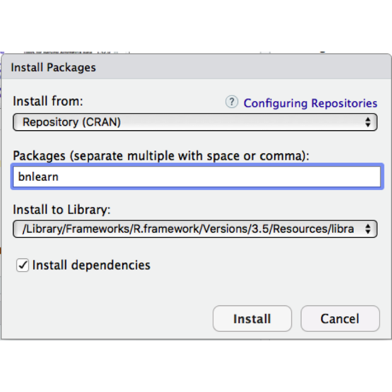
3.1 Installing bnlearn
Open RStudio and in console type:
install.packages(bnlearn)
install.packages(Rgraphviz)
If you experience problems installing Rgraphviz, try the following script:
if (!requireNamespace("BiocManager", quietly = TRUE))
    install.packages("BiocManager")
BiocManager::install("Rgraphviz")
Then type “bnlearn” in the window that appears and click on the install button. Do the same thing for the other package.
3.2 Understanding the directed acyclic graph representation
In this part, we introduce survey data set and show how we can visualize it with bnlearn package.
3.2.1 The survey data dataset
Survey data is a data set that contains information about usage of different transportation systems with a focus on cars and trains for different social groups. It includes these factors:
Age (A): It is recorded as young (young) for individuals below 30 years, adult (adult) for individuals between 30 and 60 years old, and old (old) for people older than 60.
Sex (S): The biological sex of individual, recorded as male (M) or female (F).
Education (E): The highest level of education or training completed by the individual, recorded either high school (high) or university degree (uni).
Occupation (O): It is recorded as an employee (emp) or a self employed (self) worker.
Residence (R): The size of the city the individual lives in, recorded as small (small) or big (big).
Travel (T): The means of transport favoured by the individual, recorded as car (car), train (train) or other (other)
Travel is the target of the survey, the quantity of interest whose behaviour is under investigation.
3.2.2 Visualizing a Bayesian network
We can represent the relationships between the variables in the survey data by a directed graph where each node correspond to a variable in data and each edge represents conditional dependencies between pairs of variables.
In bnlearn, we can graphically represent the relationships between variables in survey data like this:
# empty graph
library(bnlearn)
## Warning: package 'bnlearn' was built under R version 3.5.2##
## Attaching package: 'bnlearn'## The following objects are masked from 'package:BiocGenerics':
##
## path, score## The following object is masked from 'package:stats':
##
## sigmadag <- empty.graph(nodes = c("A","S","E","O","R","T"))
arc.set <- matrix(c("A", "E",
"S", "E",
"E", "O",
"E", "R",
"O", "T",
"R", "T"),
byrow = TRUE, ncol = 2,
dimnames = list(NULL, c("from", "to")))
arcs(dag) <- arc.set
nodes(dag)## [1] "A" "S" "E" "O" "R" "T"arcs(dag)## from to
## [1,] "A" "E"
## [2,] "S" "E"
## [3,] "E" "O"
## [4,] "E" "R"
## [5,] "O" "T"
## [6,] "R" "T"3.2.3 Plotting the DAG
In this section we discuss the ways that we can visually demonstrate Bayesian networks.
You can either use the simple plot function or use the graphviz.plot function from Rgraphviz package.
# plot dag with plot function
plot(dag)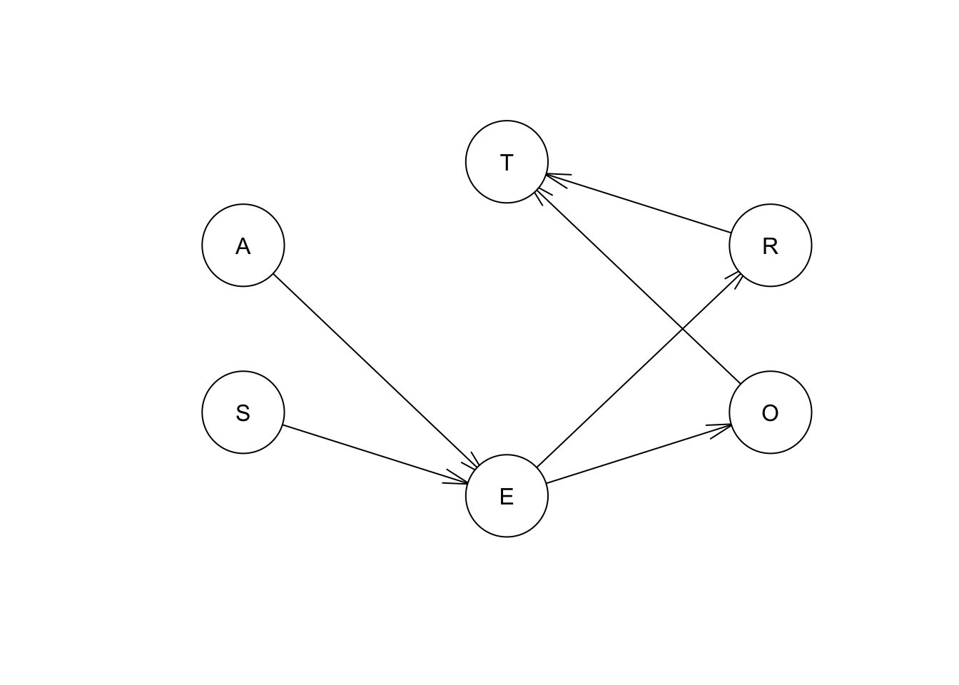
# plot dag with graphviz.plot function. Default layout is dot
graphviz.plot(dag, layout = "dot")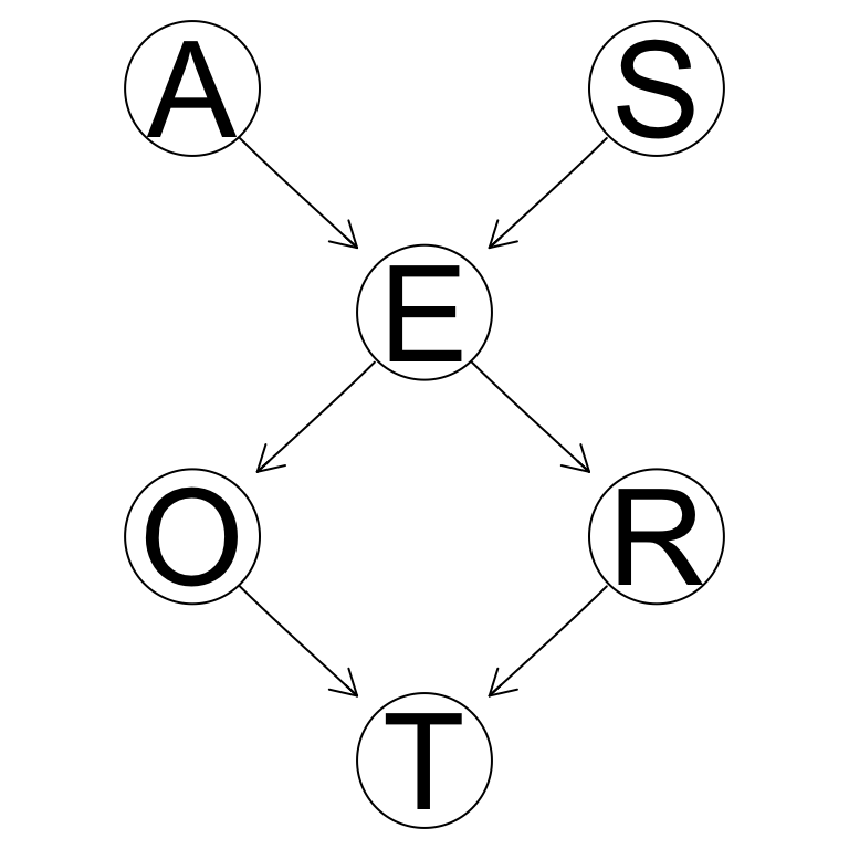
# plot dag with graphviz.plot function. change layout to "fdp"
graphviz.plot(dag, layout = "fdp")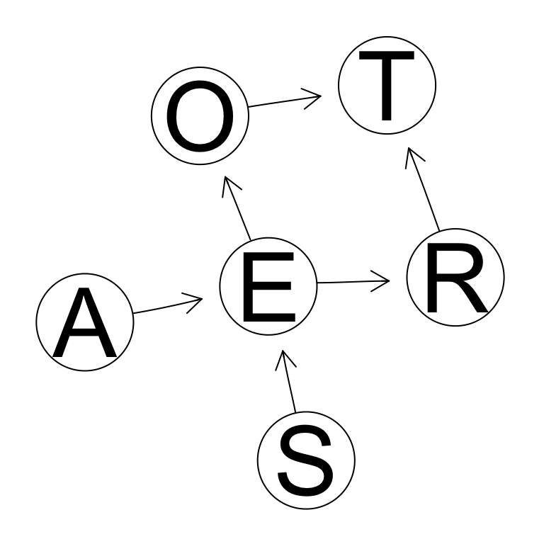
# plot dag with graphviz.plot function. change layout to "circo"
graphviz.plot(dag, layout = "circo")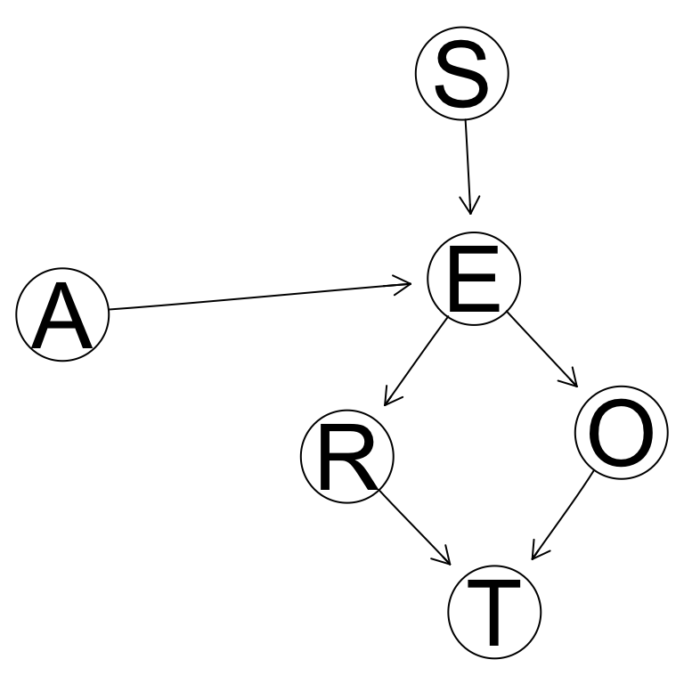
3.2.4 Highlighting specific nodes
If you want to change the color of the nodes or the edges of your graph, you can do this easily by adding a highlight input to the graphviz.plot function.
Let’s assume that we want to change the color of all the nodes and edges of our dag to blue.
hlight <- list(nodes = nodes(dag), arcs = arcs(dag),
               col = "blue", textCol = "blue")
pp <- graphviz.plot(dag, highlight = hlight)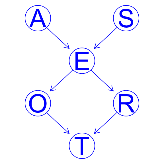
The look of the arcs can be customised as follows using the edgeRenderInfo function from Rgraphviz.
edgeRenderInfo(pp) <- list(col = c("S~E" = "black", "E~R" = "black"),
                           lwd = c("S~E" = 3, "E~R" = 3))
Attributes being modified (i.e., col for the colour and lwd for the line width) are specified again as the elements of a list. For each attribute, we specify a list containing the arcs we want to modify and the value to use for each of them. Arcs are identified by labels of the form parent∼child, e.g., S → E is S~E.
Similarly, we can highlight nodes with nodeRenderInfo. We set their colour and the colour of the node labels to black and their background to grey.
nodeRenderInfo(pp) <- list(col = c("S" = "black", "E" = "black", "R" = "black"),
                           fill = c("E" = "grey"))
Once we have made all the desired modifications, we can plot the DAG again with the renderGraph function from Rgraphviz.
renderGraph(pp)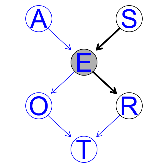
3.2.5 The directed acyclic graph as a representation of joint probability
The DAG represents a factorization of the joint probability distribution into a joint probability distribution. In this section we show how to add custom probability distributions to a DAG, as well as how to estimate the parameters of the conditional probability distribution using maximum likelihood estimation or Bayesian estimation.
3.2.6 Specifying the probability distributions on your own
Given the DAG, the joint probability distribution of the survey data variables factorizes as follows:
\(Pr(A, S, E, O, R, T) = Pr(A) Pr(S) Pr(E | A, S) Pr(O | E) Pr(R | E) Pr(T | O, R).\)
A.lv <- c("young", "adult", "old")
S.lv <- c("M", "F")
E.lv <- c("high", "uni")
O.lv <- c("emp", "self")
R.lv <- c("small", "big")
T.lv <- c("car", "train", "other")

A.prob <- array(c(0.3,0.5,0.2), dim = 3, dimnames = list(A = A.lv))
S.prob <- array(c(0.6,0.4), dim = 2, dimnames = list(S = S.lv))
E.prob <- array(c(0.75,0.25,0.72,0.28,0.88,0.12,0.64,0.36,0.70,0.30,0.90,0.10), dim = c(2,3,2), dimnames = list(E = E.lv, A = A.lv, S = S.lv))
O.prob <- array(c(0.96,0.04,0.92,0.08), dim = c(2,2), dimnames = list(O = O.lv, E = E.lv))
R.prob <- array(c(0.25,0.75,0.2,0.8), dim = c(2,2), dimnames = list(R = R.lv, E = E.lv))
T.prob <- array(c(0.48,0.42,0.10,0.56,0.36,0.08,0.58,0.24,0.18,0.70,0.21,0.09), dim = c(3,2,2), dimnames = list(T = T.lv, O = O.lv, R = R.lv))
cpt <- list(A = A.prob, S = S.prob, E = E.prob, O = O.prob, R = R.prob, T = T.prob)
# custom cpt table
cpt## $A
## A
## young adult old
## 0.3 0.5 0.2
##
## $S
## S
## M F
## 0.6 0.4
##
## $E
## , , S = M
##
## A
## E young adult old
## high 0.75 0.72 0.88
## uni 0.25 0.28 0.12
##
## , , S = F
##
## A
## E young adult old
## high 0.64 0.7 0.9
## uni 0.36 0.3 0.1
##
##
## $O
## E
## O high uni
## emp 0.96 0.92
## self 0.04 0.08
##
## $R
## E
## R high uni
## small 0.25 0.2
## big 0.75 0.8
##
## $T
## , , R = small
##
## O
## T emp self
## car 0.48 0.56
## train 0.42 0.36
## other 0.10 0.08
##
## , , R = big
##
## O
## T emp self
## car 0.58 0.70
## train 0.24 0.21
## other 0.18 0.09Now that we have defined both the DAG and the local distribution corresponding to each variable, we can combine them to form a fully-specified BN. We combine the DAG we stored in dag and a list containing the local distributions, which we will call cpt, into an object of class bn.fit called bn.
# fit cpt table to network
bn <- custom.fit(dag, cpt)
3.3 Estimating parameters of conditional probability tables
For the hypothetical survey described in this chapter, we have assumed to know both the DAG and the parameters of the local distributions defining the BN. In this scenario, BNs are used as expert systems, because they formalise the knowledge possessed by one or more experts in the relevant fields. However, in most cases the parameters of the local distributions will be estimated (or learned) from an observed sample.
Let’s read the survey data:
survey <- read.table("data/survey.txt", header = TRUE)
head(survey)
## A R E O S T
## 1 adult big high emp F car
## 2 adult small uni emp M car
## 3 adult big uni emp F train
## 4 adult big high emp M car
## 5 adult big high emp M car
## 6 adult small high emp F trainIn the case of this survey, and of discrete BNs in general, the parameters to estimate are the conditional probabilities in the local distributions. They can be estimated, for example, with the corresponding empirical frequencies in the data set, e.g.,
\(\hat{Pr}(O = emp | E = high) = \frac{\hat{Pr}(O = emp, E = high)}{\hat{Pr}(E = high)}= \frac{\text{number of observations for which O = emp and E = high}}{\text{number of observations for which E = high}}\)
This yields the classic frequentist and maximum likelihood estimates. In bnlearn, we can compute them with the bn.fit function. bn.fit complements the custom.fit function we used in the previous section; the latter constructs a BN using a set of custom parameters specified by the user, while the former estimates the same from the data.
bn.mle <- bn.fit(dag, data = survey, method = "mle")
bn.mle
##
## Bayesian network parameters
##
## Parameters of node A (multinomial distribution)
##
## Conditional probability table:
## adult old young
## 0.472 0.208 0.320
##
## Parameters of node S (multinomial distribution)
##
## Conditional probability table:
## F M
## 0.402 0.598
##
## Parameters of node E (multinomial distribution)
##
## Conditional probability table:
##
## , , S = F
##
## A
## E adult old young
## high 0.6391753 0.8461538 0.5384615
## uni 0.3608247 0.1538462 0.4615385
##
## , , S = M
##
## A
## E adult old young
## high 0.7194245 0.8923077 0.8105263
## uni 0.2805755 0.1076923 0.1894737
##
##
## Parameters of node O (multinomial distribution)
##
## Conditional probability table:
##
## E
## O high uni
## emp 0.98082192 0.92592593
## self 0.01917808 0.07407407
##
## Parameters of node R (multinomial distribution)
##
## Conditional probability table:
##
## E
## R high uni
## big 0.7178082 0.8666667
## small 0.2821918 0.1333333
##
## Parameters of node T (multinomial distribution)
##
## Conditional probability table:
##
## , , R = big
##
## O
## T emp self
## car 0.58469945 0.69230769
## other 0.19945355 0.15384615
## train 0.21584699 0.15384615
##
## , , R = small
##
## O
## T emp self
## car 0.54700855 0.75000000
## other 0.07692308 0.25000000
## train 0.37606838 0.00000000Note that we assume we know the structure of the network, so dag is an input of bn.fit function.
As an alternative, we can also estimate the same conditional probabilities in a Bayesian setting, using their posterior distributions. In this case, the method argument of bn.fit must be set to “bayes”.
bn.bayes <- bn.fit(dag, data = survey, method = "bayes", iss = 10)The estimated posterior probabilities are computed from a uniform prior over each conditional probability table. The iss optional argument, whose name stands for imaginary sample size (also known as equivalent sample size), determines how much weight is assigned to the prior distribution compared to the data when computing the posterior. The weight is specified as the size of an imaginary sample supporting the prior distribution.
3.3.1 Fit dag to data and predict the value of latent variable
# predicting a variable in the test set.
training = bn.fit(model2network("[A][B][E][G][C|A:B][D|B][F|A:D:E:G]"),
                  gaussian.test[1:2000, ])
test = gaussian.test[2001:nrow(gaussian.test), ]
predicted <- predict(training, node = "A", data = test, method = "bayes-lw")
head(predicted)
## [1] 3.2905037 0.5755309 0.6127167 1.7173029 1.0264255 1.0253681about the method bayes-lw: the predicted values are computed by averaging likelihood weighting simulations performed using all the available nodes as evidence (obviously, with the exception of the node whose values we are predicting). If the variable being predicted is discrete, the predicted level is that with the highest conditional probability. If the variable is continuous, the predicted value is the expected value of the conditional distribution.
3.4 Conditional independence in Bayesian networks
Using a DAG structure we can investigate whether a variable is conditionally independent from another variable given a set of variables from the DAG. If the variables depend directly on each other, there will be a single arc connecting the nodes corresponding to those two variables. If the dependence is indirect, there will be two or more arcs passing through the nodes that mediate the association.
If \(\textbf{X}\) and \(\textbf{Y}\) are separated by \(\textbf{Z}\), we say that \(\textbf{X}\) and \(\textbf{Y}\) are conditionally independent given \(\textbf{Z}\) and denote it with,
\[\textbf{X } { \!\perp\!\!\!\perp}_{G} \textbf{Y } | \textbf{ Z}\] Conditioning on \(\textbf{Z}\) is equivalent to fixing the values of its elements, so that they are known quantities.
\(\textbf{Definition (MAPS).}\) Let M be the dependence structure of the probability distribution P of data \(\textbf{D}\), that is, the set of conditional independence relationships linking any triplet \(\textbf{X}\), \(\textbf{Y}\), \(\textbf{Z}\) of subsets of \(\textbf{D}\). A graph G is a dependency map (or D-map) of M if there is a one-to-one correspondence between the random variables in \(\textbf{D}\) and the nodes \(\textbf{V}\) of G such that for all disjoint subsets \(\textbf{X}\), \(\textbf{Y}\), \(\textbf{Z}\) of \(\textbf{D}\) we have
\[\textbf{X } {\!\perp\!\!\!\perp}_{P} \textbf{ Y } | \textbf{ Z} \Longrightarrow \textbf{X } {\!\perp\!\!\!\perp}_{G} \textbf{ Y } | \textbf{ Z}\]
Similarly, G is an independency map (or I-map) of M if
\[\textbf{X } {\!\perp\!\!\!\perp}_{P} \textbf{ Y } | \textbf{ Z} \Longleftarrow \textbf{X } {\!\perp\!\!\!\perp}_{G} \textbf{ Y } | \textbf{ Z}\] G is said to be a perfect map of M if it is both a D-map and an I-map, that is
\[\textbf{X } {\!\perp\!\!\!\perp}_{P} \textbf{ Y } | \textbf{ Z} \Longleftrightarrow \textbf{X } {\!\perp\!\!\!\perp}_{G} \textbf{ Y } | \textbf{ Z}\] and in this case G is said to be faithful or isomorphic to M.
\(\textbf{Definition.}\) A variable V is a collider or has a V structure, if it has 2 upcoming parents.
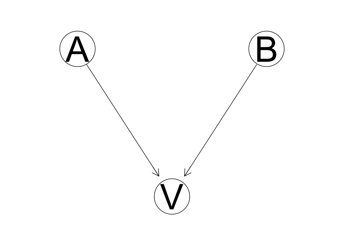
(#fig:02_colider_net)V is a collider
You can find all the V structures of a DAG:
vstructs(dag)## X Z Y
## [1,] "A" "E" "S"
## [2,] "O" "T" "R"Note that conditioning on a collider induces dependence even though the parents aren’t directly connected.
\(\textbf{Definition (d-separation)}\) If G is a directed graph in which \(\textbf{X}\), \(\textbf{Y}\) and \(\textbf{Z}\) are disjoint sets of vertices, then \(\textbf{X}\) and \(\textbf{Y}\) are d-connected by \(\textbf{Z}\) in G if and only if there exists an undirected path U between some vertex in \(\textbf{X}\) and some vertex in \(\textbf{Y}\) such that for every collider C on U, either C or a descendent of C is in \(\textbf{Z}\), and no non-collider on U is in \(\textbf{Z}\).
\(\textbf{X}\) and \(\textbf{Y}\) are d-separated by \(\textbf{Z}\) in G if and only if they are not d-connected by \(\textbf{Z}\) in G.
We assume that graphical separation (\({\!\perp\!\!\!\perp}_{G}\)) implies probabilistic independence (\({\!\perp\!\!\!\perp}_{P}\)) in a Bayesian network.
We can investigate whether two nodes in a bn object are d-separated using the dsep function. dsep takes three arguments, x, y and z, corresponding to \(\textbf{X}\), \(\textbf{Y}\) and \(\textbf{Z}\); the first two must be the names of two nodes being tested for d-separation, while the latter is an optional d-separating set. So, for example,
dsep(dag, x = "S", y = "R")## [1] FALSEdsep(dag, x = "O", y = "R")## [1] FALSEdsep(dag, x = "S", y = "R", z = "E")## [1] TRUE3.4.1 Markov Property, Equivalence classes and CPDAGS
\(\textbf{Definition (Local Markov property)}\) Each node \(X_i\) is conditionally independent of its non-descendants given its parents.
Compared to the previous decomposition, it highlights the fact that parents are not completely independent from their children in the BN; a trivial application of Bayes’ theorem to invert the direction of the conditioning shows how information on a child can change the distribution of the parent.
Second, assuming the DAG is an I-map also means that serial and divergent connections result in equivalent factorisations of the variables involved. It is easy to show that
\[\begin{align} Pr(X_i) Pr(X_j | X_i) Pr(X_k | X_j) &= Pr(X_j,X_i) Pr(X_k | X_j)\\ &= Pr(X_i | X_j) Pr(X_j) Pr(X_k | X_j) \end{align}\]Then \(X_i \longrightarrow X_j \longrightarrow X_k\) and \(X_i \longleftarrow X_j \longrightarrow X_k\) are equivalent. As a result, we can have BNs with different arc sets that encode the same conditional independence relationships and represent the same global distribution in different (but probabilistically equivalent) ways. Such DAGs are said to belong to the same equivalence class.
3.4.2 Skeleton of a network, CPDAGs and equivalence classes
The skeleton of a network is the network without any direction. Here is the skeleton of the dag for survey dataset.
graphviz.plot(skeleton(dag))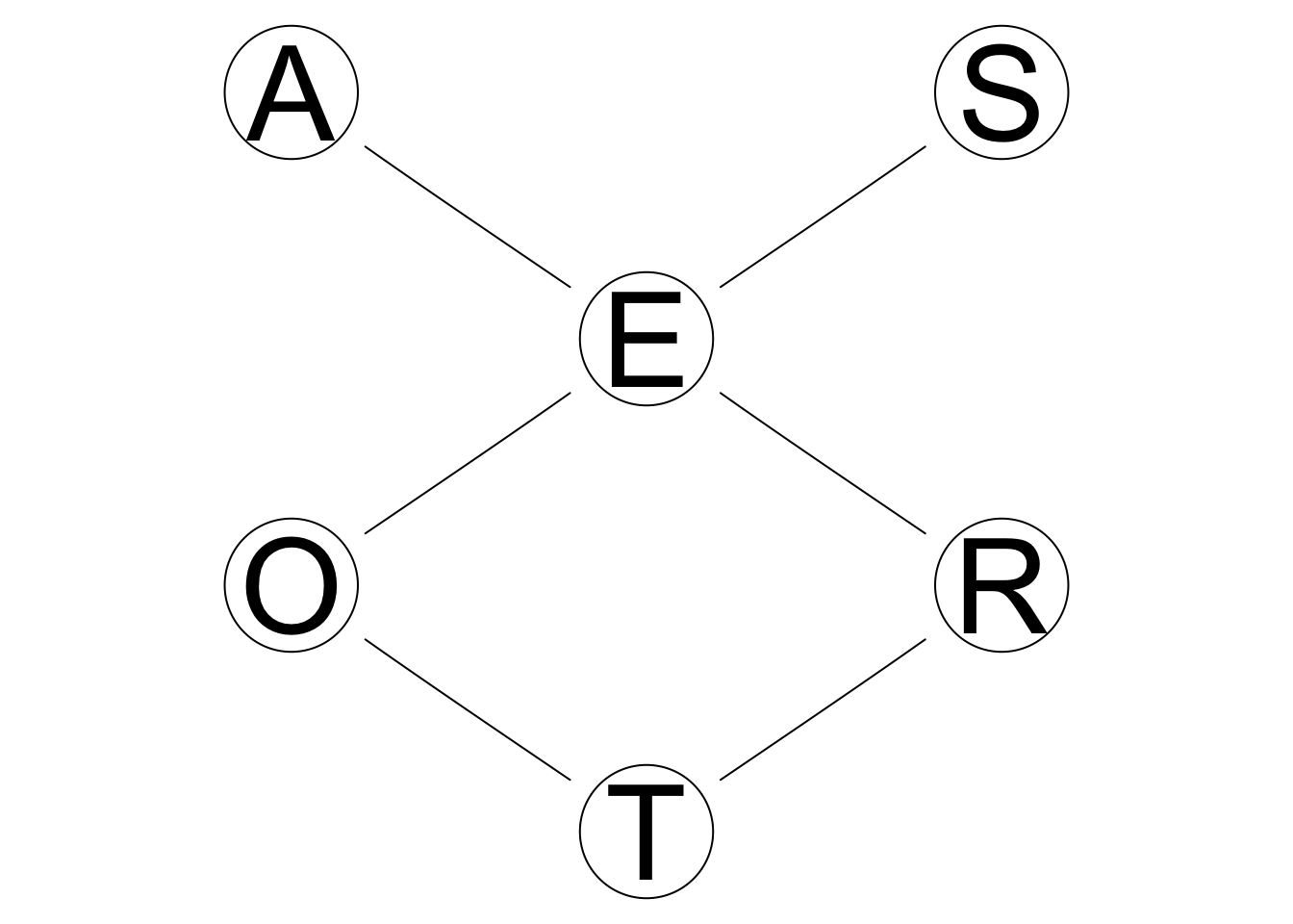
\(\textbf{Theorem. (Equivalence classes)}\) Two DAGs defined over the same set of variables are equivalent and only they have the same skeleton (i.e., the same underlying undirected graph) and the same v-structures.
data(learning.test)
learn.net1 = empty.graph(names(learning.test))
learn.net2 = empty.graph(c("A","B","C","D","E","F"))
modelstring(learn.net1) = "[A][C][F][B|A][D|A:C][E|B:F]"
arc.set2 <- matrix(c("B", "A",
                    "A", "D",
                    "C", "D",
                    "B", "E",
                    "F", "E"),
                  byrow = TRUE, ncol = 2,
                  dimnames = list(NULL, c("from", "to")))
arcs(learn.net2) <- arc.set2
graphviz.compare(learn.net1,learn.net2)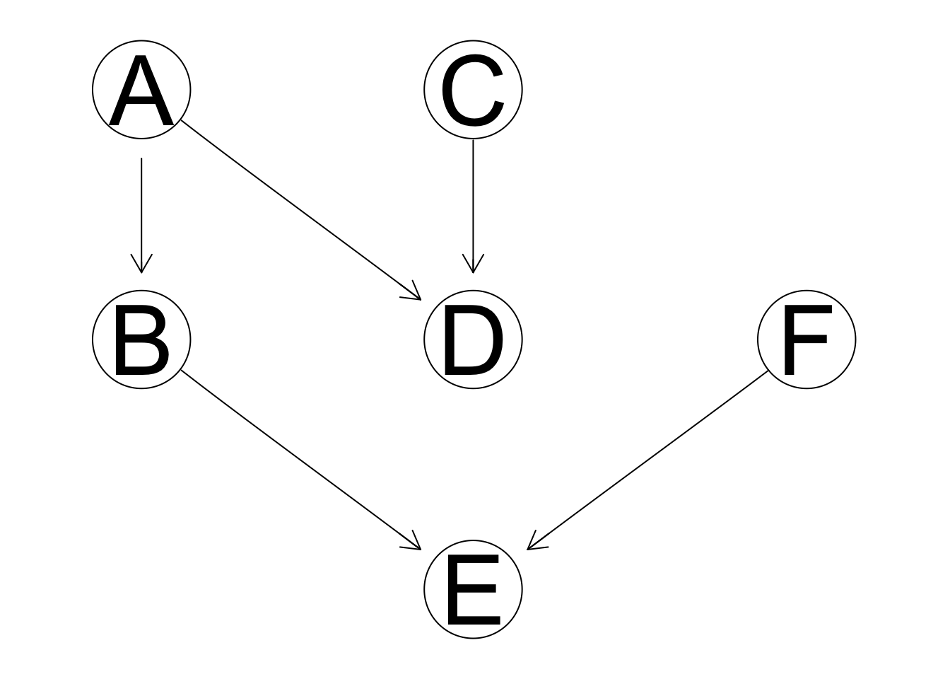
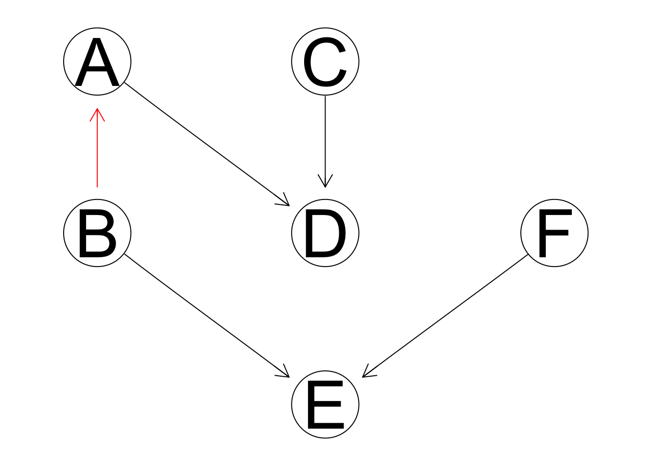
score(learn.net1, learning.test, type = "loglik")## [1] -23832.13score(learn.net2, learning.test, type = "loglik")## [1] -23832.13# type == "loglik" means you get the log likelihood of the data given the dag and the MLE of the parametersIn other words, the only arcs whose directions are important are those that are part of one or more v-structures.
The skeleton of a DAG and it’s V structures identify the equivalence class the DAG belongs to, which is represented by the completed partially directed graph (CPDAG). We can obtain it from a DAG with cpdag function.
X <- paste("[X1][X3][X5][X6|X8][X2|X1][X7|X5][X4|X1:X2]",
           "[X8|X3:X7][X9|X2:X7][X10|X1:X9]", sep = "")
dag2 <- model2network(X)
par(mfrow = c(1,2))
graphviz.plot(dag2)
graphviz.plot(cpdag(dag2))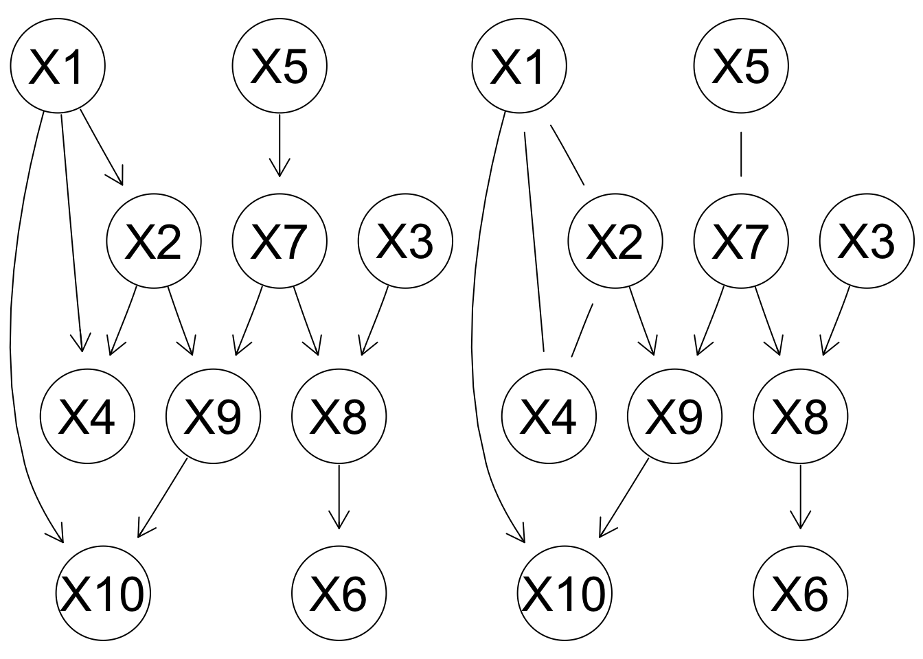
3.4.3 Moral Graphs
In previous Section we introduced an alternative graphical representation of the DAG underlying a BN: the CPDAG of the equivalence class the BN belongs to. Another graphical representation that can be derived from the DAG is the moral graph.
The moral graph is an undirected graph that is constructed as follows:
connecting the non-adjacent nodes in each v-structure with an undirected arc;
ignoring the direction of the other arcs, effectively replacing them with undirected arcs.
This transformation is called moralisation because it “marries” non-adjacent parents sharing a common child. In the case of our example dag, we can create the moral graph with the moral function as follows:
graphviz.plot(moral(dag2))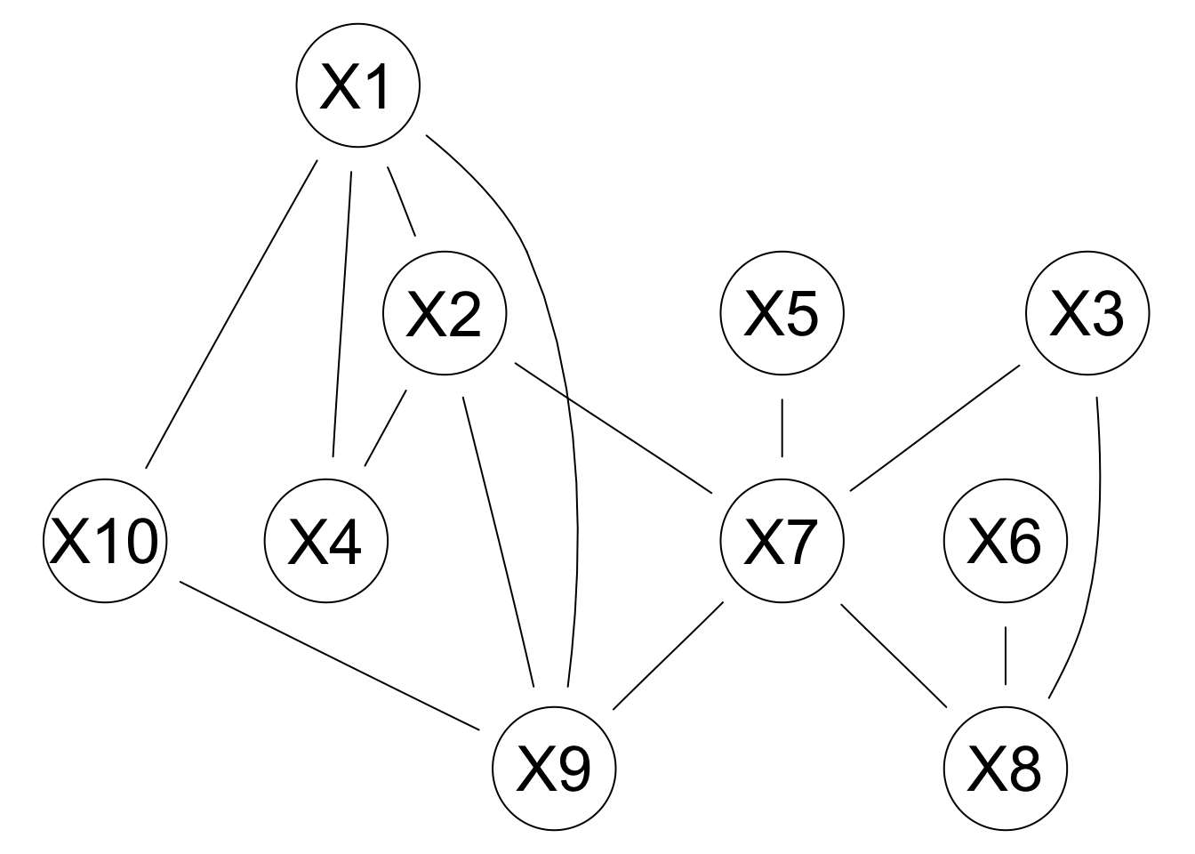
Moralisation has several uses. First, it provides a simple way to transform a BN into the corresponding Markov network, a graphical model using undirected graphs instead of DAGs to represent dependencies.
In a Markov network, we say that \(\textbf{X} {\!\perp\!\!\!\perp}_{G} \textbf{Y} | \textbf{Z}\) if every path between \(\textbf{X}\) and \(\textbf{Y}\) contains some node \(Z \in \textbf{Z}\).
3.5 Plotting Conditional Probability Distributions
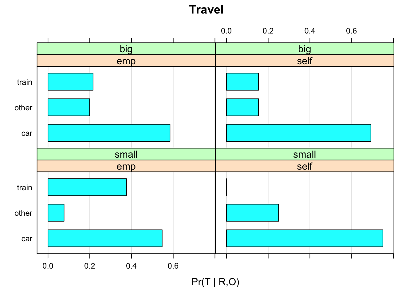
Plotting the conditional probabilities associated with a conditional probability table or a query is also useful for diagnostic and exploratory purposes. Such plots can be difficult to read when a large number of conditioning variables is involved, but nevertheless they provide useful insights for most synthetic and real-world data sets.
As far as conditional probability tables are concerned, bnlearn provides functions to plot barcharts (bn.fit.barchart) and dot plots (bn.fit.dotplot) from bn.fit objects. Both functions are based on the lattice package. For example let’s look at the conditional plot of \(Pr(T | R,O)\):
bn.fit.barchart(bn.mle$T, main = "Travel",
                xlab = "Pr(T | R,O)", ylab = "")
## Loading required namespace: lattice