8 Confounding, Paradoxes
8.1 A second look at confounding
- Confounding
- Interested in an average treatment effect.
- In context of randomized A/B, this is the difference on average between outcome under group A and outcome under group B
- More generally, the average difference between interventions.
- So we want this intervention distribution.
- The adjustment criterion tell us what variables we can control for.
- We think of these in terms of sets, because some confounders may be hidden.
- It may not be possible to control for everythings
- The adjustment formula tells us that once we have the covariate-adjustment formula, we can estimate this intervention distribution.
8.2 Monte Hall
- Describe problem
- Game show
- Choose a door
- Monte will open a door that does not have the car
- Should always pick.
- Monty Hall must open a door that does not have a car behind it
- chosen door -> door open <- location of the car (scribe create figure)
- Door opened is a collider
8.3 Berkson Paradox
- Two features seem to have no relation to each other in general, they can appear to be associated within a context
- This is the core of sampling bias
8.4 Examples of valid adjustment
8.5 Covariate adjustment: Simpson’s Paradox
You are a data scientist at a prominent tech company with paid subscription entertainment media streaming service. You come across there results of an A/B test that a rival data scientist ran. The test targeted 70K subscibers users who were coming to a subscription renewal time and were at high risk of not renewing. They were targeted with either treatment 0 - a personalized promotional offer that gave the user reduced rates on the media they consume the most, or treatment 1 - a promotional offer that gave the user reduced rates on a general set of content.
| Overall | |
|---|---|
| Treatment 0: Personalized Promotion | 77.9% (27272/35000) |
| Treatment 1: Generalized Promotion | 82.6% (28902/35000) |
This reads that 78% of the users who recieved the personalized promotion ended up renewing their subscription, while 83% of those who recieved the generalized promotion ended up renewing.
Let R be the 0 if a subscriber leaves, and 1 if a subsciber stays. In his report, the analyst quantified the effect size as:
\[ E(R | T = 0) - E(R | T = 1) = P(R = 1 | T = 0) - P(R = 1 | T = 1) \approx .779 - .826 = -0.047 \]
… where .779 and .826 are empirical estimates. So the conclusion was that the probability a subscriber stays is nearly .05 higher on the generalized promotion than on the personalized promotion.
The marketing executives took this as a no-brainer. While the effect size is small, the p-value was near 0 so these results were significant (never mind that this was simply because sample size is large, which is typically the case in tech). Users generally prefer high quality content, and high quality content generally has higher royalty costs. So personalized promotions are typically more expensive than the generalized ones, where you can mix less popular but more cost-effective content into the promotion. So if the generalized promotion is cheaper AND performs better in the test, then its clearly better choice as a policy for dealing with subscribers who at high risk of leaving… Right?
Curious, you find the SQL query that generated the data, and play around with selecting a few more columns and joining a few other tables. You notice that for these subscribes, there was also data on how happy the customers were, based on interactions with customer service. You create a new table that works in this new Z(not disgruntled/disgruntled) variable.
| Overall | Not disgruntled | Disgruntled | |
|---|---|---|---|
| Treatment 0: Personalized Promotion | 77.9% (27272/35000) | 93.2% (8173/8769) | 73.3% (19228/26231) |
| Treatment 1: Generalized Promotion | 82.6% (28902/35000) | 86.9% (23339 / 26872) | 68.7% (5582/8128) |
Lo and behold, the conclusion is reversed within each level of Z! While generalized promotion seems favorable relative to personalized promotion in general, the personalized promotion seems to perform better within each of the non-disgruntled and disgruntled subgroups. This turns out to be an example of Simpon’s paradox.
Suppose the true underlying model has the following DAG:

simpson_model
…where Z is 0 for non-disgruntled, 1 if disgruntled.
Consider two SCMs \(\mathbb{C}^{do(T:=0)}\) and \(\mathbb{C}^{do(T:=0)}\) that are obtained by interventions setting \(T := 0\) and \(T := 1\). Let \(P^{\mathbb{C};do(T:=0)}\) and \(P^{\mathbb{C};do(T:=0)}\) denote the probability distributes entailed by these SCMs.
Calculate the expected difference in outcome between the two treatments using the empirical counts in the above table $ E^{T=0}(R) - E^{T=1}(R)$.
Calculate analytical the Average Treatment Effect using the empirical values in the table:
\[ \begin{align*} ATE &= E^{do(T:=0)}(R) - E^{do(T:=1)}(R)\\ &= P^{\mathbb{C};do(T:=0)}(R=1) - P^{\mathbb{C};do(T:=1)}(R-1)\\ \ \\ P^{\mathbb{C};do(T:=0)}(R=1) &= \sum_{z=0}^1 P^{\mathbb{C};do(T:=0)}(R=1, Z=z) \\ &= \sum_{z=0}^1 P^{\mathbb{C};do(T:=0)}(R=1, T=0, Z=z) \\ &= \sum_{z=0}^1 P^{\mathbb{C};do(T:=0)}(R=1| T=0, Z=z) P^{\mathbb{C};do(T:=0)}(T=0, Z=z) \\ &= \sum_{z=0}^1 P^{\mathbb{C};do(T:=0)}(R=1| T=0, Z=z) P^{\mathbb{C};do(T:=0)}(Z=z) \\ &= \sum_{z=0}^1 P^{\mathbb{C}}(R=1| T=0, Z=z) P^{\mathbb{C}}(Z=z) \\ &\approx .932 * 35641/70000 + .733 * 34359/70000 = .8343 \ \\ P^{\mathbb{C};do(T:=1)}(R=1) &\approx .869 * 35641/70000 + .687 * 34359/70000 = .7818 \ \\ \ \\ ATE &= .8343 - .7818 = 0.0525\\ \end{align*} \]
8.6 Front-door adjustment
- Front-door criterion: A set of variables Z is siad to satisfy the front-door criterion relative to an ordered pair of variables (X, Y) if
- Z intercepts all directed paths from X to Y
- There are no unblocked paths from X to Z
All backdoor paths from Z to Y are blocked by X
- You are a data scientist investing the effects of social media use on a purchase.
- You assume the following DAG
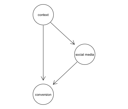
- Circles mean unobserved, squares mean observed
- In this model the causal effect of social media on conversions is not identifiable; one can never ascertain which portion of the observed correlation between X and Y is attributed to user context U.
- It is worth noting that there are ways of analyzing how strong that confounding effects must be in order to entirely explain the association between X and Y
- Now suppose you modify the SQL query and get an additional variable: whether or not the person was using an ad blox.
- In this case we can apply the front-door criterion.
- Assume that were query the database for a past experiment where a randomly selected sample of 800000 “whales” – tech lingo for users who generally have a high conversion rate (because of evironmental factors, like their generation or social/professional in-group).
- Assume the following tqble (blackboard)
- One person on your team argues that the table proves that social media does not drive conversions. They point to the fact that only 15% of people who converted used social media, compared to 92.25% of people who don’t use social media.
- Another member oof your team argues that social media use actual increases, not decreases, conversions.
- Their argument is as follows: If you use social media, then your chances of seeing a high level of ads is 95% (380/400) compared to 5% if you do not use social media (20/400).
- The effect of ad exposure, if we look seperately at the two groups, social media users and non-users in in the second table (blackboard).
- In social media users it increases conversion rates from 10% to 15%
- in non-social media users it increases conversion rates from 90 to 95%
- Here is how we break the stalemate with a technique called the front-door formula:
- First, we see that the effect of X on Z is identifiable because there is no backdoor path from Z to X. \(P(Z = z|do(X = x))\) = P(Z = z|X = x)
- Next, we not that the effect of Z on Y is identifiable. The backdow path from Z to Y, namely Z <- X <- U -> Y can conditioning on X. \(P(Y = y|do(Z = z)) = \sum_x P(Y = y|Z = z, X=x)P(X = x)\)
- We chain toghether these two parital effects to obtain the overall effect of X on Y.
- If nature chooses to assign Z the value z, then the probability of Y would be \(P(Y=y | do(Z = z))\).
- The probability that nature would choose to do that, given that we choose to set X to x is \(P(Z = z|do(X = x))\)
- Summing up over all the possible states z of Z we have \[ P(Y = y|do(X = x)) = \sum_Z P(Y = y |do(Z = z))P(Z =z|do(X = x)) \]
- Finally, we replace the do-expressions with their covariate adjustment counterparts. The final expression is \[P(Y = y|do(X = x)) = \sum \sum_{x'} P(Y = y|Z = z, X = x')P(X = x')P(Z = z|X = x)\]
8.7 Propensity score
- Consider the following case of confounding:
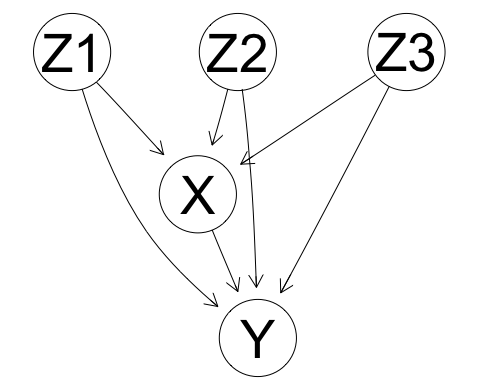
- The set {Z1, Z2, Z3} is a valid adjustment set by parent adjustment
- So we could estimate the intervention distribution using \(p^{M; do(X:=x)}(y) = \sum_{z_1, z_2, z_3}p^{\mathbb{M}}(y|x, z_1, z_2, z_3)p^{\mathbb{M}}(z_1, z_2, z_3)\)
- Here we consider the case where Z1, Z2, and Z3 there exists some function \(L(Z_1, Z_2, Z_3)\) that renders X conditionally independent from Z1, Z2, Z3, i.e. $ X{ Z_1, Z_2, Z_3 } |L(Z_1, Z_2, Z_3)$
- To help imagine this, it modify our causal model to add \(L(Z_1, Z_2, Z_3)\) to the graph as a type of continuous causal AND gate as in
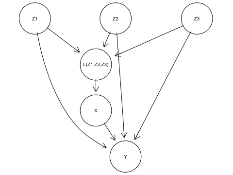 .
. - Let \(l\) represent a value codomain of \(L(.)\)
- Our new adjustment formula is \(p^{M; do(X:=x)}(y) = \sum_{l}p^{\mathbb{M}}(y|x, l)p^{\mathbb{M}}(l)\)
- What have we gained here? \(p(y |x, l)\) is potentially of lower dimention that \(p(y|x, z_1, z_2, z_3)\). It might be computationally easier to estimate \(p^{M; do(X:=x)}(y)\) with covariate adjustment over \(L(.)\) than over Z1, Z2, Z3.
- In industry and practice, you often hear of “propensity matching”, where you try to group examples that have similar values of \(L(.)\) and then calculste cause effects between X and Y within those groups. In other words, you control for/condition on/adjust for L
Next class (scribes delete) * Structural causal models * Instrumental variables * Potential outcomes * Inverse proability weighting * mediation