Other stuff
Recap
- On the difference between covariate adjustment and do-calculus
- Covariate adjustment allows us to predict the results of an intervention.
- Requires we observe the variables required to do the adjustment
- Covariate adjustment is taking a weighted average of an effect over every combination of strata in the adjustment set. This is practically difficult (in terms of computation and expectation) if the number of strata is large. If Z is continuous, then you have to integrate, which has its own set of practical challenges.
- Do-calculus is simulation of an intervention
- When you don’t have the variables neccessary to do covariate adjustment, you can still use do-calculus
How to simulating adjustment using a propensity score function and inverse probability weighting
- This is useful when adjusting over all the strata in the adjustment set is practically difficult
- Adjustment formula: \[P(Y=y|do(X = x)) = \sum_{Z} P(Y= y|X = x, Z = z)P(Z = z)\]
- Looking just at \(P(Y= y|X = x, Z = z)\), Baye’s rule tells us that: \[P(Y= y|X = x, Z = z) = \frac{P(X = x, Y= y, Z = z)}{P(X = x, Z = z)}\]
- Bring back \(P(Z = z)\)
\[\begin{align}
P(Y= y|X = x, Z = z)P(Z=z) &= \frac{P(X = x, Y= y, Z = z)}{P(X = x, Z = z)}P(Z=z) \\
&= \frac{P(X = x, Y= y, Z = z)}{P(X = x| Z = z)P(Z=z)}P(Z=z) \\
&= \frac{P(X = x, Y= y, Z = z)}{P(X = x| Z = z)}
\end{align}\]
- Therefore we can rewrite the adjustment formula as: \[P(Y=y|do(X = x)) = \sum_z \frac{P(X = x, Y= y, Z = z)}{P(X = x| Z = z)}\]
- Suppose we are able to estimate a propensity score function \(g(x, z) = P(X = x | Z = z)\)
- Then we can estimate \(P(Y = y|do(X =x))\) using the following inverse probability weighting algorithm “”" # using Pyro-ish code # M is desired number of samples samples = [] weights = [] for i in M: x, y, z = model() sample_prob = model.prob(x, y, z) propensity_score = g(x, z) weight = sample_prob / propensity_score samples.append((x, y, z)) weights.append(weight) # resample according to new weights new_samples = resample(samples, weights = weights) “”"
- It is called inverse probability weighting because you multiply the joint probability of a sample by the inverse of a probability, in this case \(g(x, z) = P(X = x|Z =z)\)
- The frequencies in
new_samples is such that you can estimate \(P(Y=y|do(X = x)\) with \(\hat{p}(Y = y|X = x)\), where \(\hat{p}\) is a proportion in new_samples.
Structural causal models
- Recall Laplace’s demon example
- As we mentioned before, a structural causal model is a deterministic extention to \(\mathbb{C}\) has a causal DAG \(\mathbb{D}\). Assume there are \(J\) random variables in the DAG.
- Each varible in the DAG is paired with on independent random variables called exogenous noise terms, I will call them noise terms
- A distribution \(P_{\mathbf{N}}^{\mathbb{C}}\) on independent random variables \(\mathbf{N} = \{N_i; i \in J \}\)
- The value of each variable is set deterministically by a function \(f_i\) for the ith random variable called a structural assignments, such that \(X_i = f_i(\mathbf{PA}_{\mathbb{C}, i}, N_i), \forall i \in J\) where \(\mathbf{PA}_{\mathbb{C}, i} \subseteq \mathbf{X} \setminus X_i\) are the parents of \(X_i\) in \(\mathbb{D}\).
- Some draw the noise terms, I usually do not.
- \(\mathbb{C}\) is a generative model that entails \(P^{\mathbb{G}}\), the same observational distribution as \(\mathbb{G}\)
- These are going to allow us to compute counterfactuals, they are on the highest rung of the ladder.
- They are not the only model on the top rung. In a subsequent class, I will introduce some generalizations of structural causal models to open universe models.
Causal inference in linear systems
- So far we have focused on covariate adjustment with discrete variables.
- We’ve avoided continuous variables generally for a few reasons.
- Setting an intervention to point on a continuous domain seems weird. Why \(do(X = 1.0)\) and not \(do(X = 1.00001)\)?
- Integration and Bayesian probability math is practically challenging.
- The math of course is simpler when you use linear modeling with Gaussian distributions. However, this class casts causal modeling as an extention of generative machine learning; in cutting-edge generative machine learning you generally don’t see a lot of linear modelling.
- However, we do touch on a few cases fundamental topics that come up in the causal linear modeling literature.
Covariate adjustment example: Continuous adjustment
- We have been talking about thinking of causal effects as differences, what might this look like in the continuous case? \(\frac{d}{dx}E^{\mathbb{M};do(X:=x)}(Y)\)
- Linear case – Z in valid adjustment set
- Nonlinear case: Monte Carlo Sampler. Recall that. \(\frac{d f(x)}{dx} = \lim_{\delta \rightarrow 0} \frac{f(x + \delta) -f(x)}{\delta}\)
Instrumental variables
- Consider a structural causal model with the following DAG
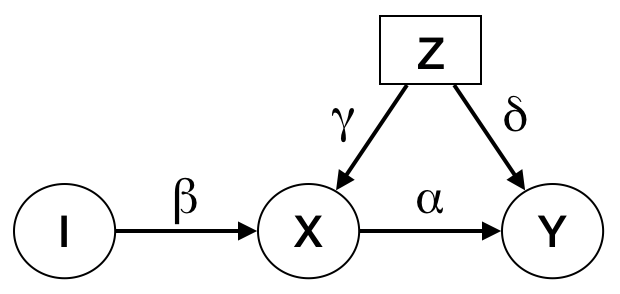
- Consider the structural assignment for Y: \(Y := \alpha X + \delta Z + N_Y\)
- We are interested in the causal effect \(\alpha\). Let \(\hat{\alpha}\) be our least-squares estimate of \(\alpha\). Here confounding shows up as a bias in the standard regression estimator \(\alpha\): \[E(\hat{\alpha}) = \frac{\text{cov}(X, Y)}{\text{var}(Y)} = \frac{\alpha \text{var}(X) + \delta \gamma \text{var}(Z)}{\text{var}(X)} = \alpha + \frac{\delta \gamma \text{var}(Z)}{\text{var}(X)} \neq \alpha \]
- An instumental variable \(I\) for \(X, Y\) is one where:
- \(I\) is independent of \(Z\)
- \(I\) is not independent of \(X\)
- \(I\) affects \(Y\) only through \(X\)
- Two-stage least squares estimation using an instrumental variable algorithm:
- Regress X on Z and get \(\hat{\beta}\) estimate of \(\beta\)
- Regress Y on the predicted values of the first regression \(\hat{\beta}Z\)
- The coefficient of \(\hat{\beta}Z\) becomes is a consistent estimate of \(\alpha\).
- Statistical intuition:
- Looking at the stuctural assignment for \(X\): \[X:= \beta I + \gamma Z + N_X\]
- Since \(Z\) and \(N_X\) are independent of \(I\), then covariance between \(Z, N_X, \hat{\gamma}\) is 0. So we can treat \(\gamma Z + N_X\) as a big noise term, and treat \(\beta Z\) as a stand in for X.
- We essentially modifiy Y’s to be : \[Y := \alpha (\beta Z) + (\alpha \gamma + \delta)Z + N_Y\] and fit it using least-squares.
Counterfactuals
- Notation
- Reasoning through inference algorithm with SMC: Eye disease model
\[\begin{align}
T &= N_T\\
B &= T * N_B + (1-T)*(1-N_B) \\
N_T ~ Ber(.5), N_B ~ Ber(.01)
\end{align}\]
- Suppose patient with poor eyesight comes to the hospital and goes blind (B=1) after the doctor gives treatment (T=1).
- We ask “what would have happened had the doctor administered treatment T = 0?”
- B = T = 1 means the \(N_B\) was 1.
- Given \(N_B\) equals 1, we calculate the effect of \(do(T = 0)\) under new model
\[\begin{align}
T &= 1\\
B &= T * 1 + (1-T)*(1-1) = T \\
\end{align}\]
Bayesian counterfactual algorithm with SMCs in Pyro
- Condition on observed data
- Infer the noise terms
- Apply do operator
- Forward from noise posterior after having applied do operation.