1.6 Working with Dates, Times, Time Zones
The learning objectives for this section are to:
- Transform non-tidy data into tidy data
- Manipulate and transform a variety of data types, including dates, times, and text data
R has special object classes for dates and date-times. It is often worthwhile to convert a column in a data frame to one of these special object types, because you can do some very useful things with date or date-time objects, including pull out the month or day of the week from the observations in the object, or determine the time difference between two values.
Many of the examples in this section use the ext_tracks object loaded earlier in the book. If you need to reload that, you can use the following code to do so:
ext_tracks_file <- "data/ebtrk_atlc_1988_2015.txt"
ext_tracks_widths <- c(7, 10, 2, 2, 3, 5, 5, 6, 4, 5, 4, 4, 5, 3, 4, 3, 3, 3,
                       4, 3, 3, 3, 4, 3, 3, 3, 2, 6, 1)
ext_tracks_colnames <- c("storm_id", "storm_name", "month", "day",
                          "hour", "year", "latitude", "longitude",
                          "max_wind", "min_pressure", "rad_max_wind",
                          "eye_diameter", "pressure_1", "pressure_2",
                          paste("radius_34", c("ne", "se", "sw", "nw"), sep = "_"),
                          paste("radius_50", c("ne", "se", "sw", "nw"), sep = "_"),
                          paste("radius_64", c("ne", "se", "sw", "nw"), sep = "_"),
                          "storm_type", "distance_to_land", "final")
ext_tracks <- read_fwf(ext_tracks_file,
                       fwf_widths(ext_tracks_widths, ext_tracks_colnames),
                       na = "-99")
1.6.1 Converting to a date or date-time class
The lubridate package (another package from the “tidyverse”) has some excellent functions for working with dates in R. First, this package includes functions to transform objects into date or date-time classes. For example, the ymd_hm function (along with other functions in the same family: ymd, ymd_h, and ymd_hms) can be used to convert a vector from character class to R’s data and datetime classes, POSIXlt and POSIXct, respectively.
Functions in this family can be used to parse character strings into dates, regardless of how the date is formatted, as long as the date is in the order: year, month, day (and, for time values, hour, minute). For example:
library(lubridate)

ymd("2006-03-12")
[1] "2006-03-12"
ymd("'06 March 12")
[1] "2006-03-12"
ymd_hm("06/3/12 6:30 pm")
[1] "2006-03-12 18:30:00 UTC"
The following code shows how to use the ymd_h function to transform the date and time information in a subset of the hurricane example data called andrew_tracks (the storm tracks for Hurricane Andrew) to a date-time class (POSIXct). This code also uses the unite function from the tidyr package to join together date components that were originally in separate columns before applying ymd_h.
library(dplyr)
library(tidyr)

andrew_tracks <- ext_tracks %>%
  filter(storm_name == "ANDREW" & year == "1992") %>%
  select(year, month, day, hour, max_wind, min_pressure) %>%
  unite(datetime, year, month, day, hour) %>%
  mutate(datetime = ymd_h(datetime))

head(andrew_tracks, 3)
# A tibble: 3 x 3
  datetime            max_wind min_pressure
  <dttm>                 <dbl>        <dbl>
1 1992-08-16 18:00:00       25         1010
2 1992-08-17 00:00:00       30         1009
3 1992-08-17 06:00:00       30         1008
class(andrew_tracks$datetime)
[1] "POSIXct" "POSIXt"
Now that the datetime variable in this dataset has been converted to a date-time class, the variable becomes much more useful. For example, if you plot a time series using datetime, ggplot2 can recognize that this object is a date-time and will make sensible axis labels. The following code plots maximum wind speed and minimum air pressure at different observation times for Hurricane Andrew (Figure 1.3)– check the axis labels to see how they’ve been formatted. Note that this code uses gather from the tidyr package to enable easy faceting, to create separate plots for wind speed and air pressure.
andrew_tracks %>%
  gather(measure, value, -datetime) %>%
  ggplot(aes(x = datetime, y = value)) +
  geom_point() + geom_line() +
  facet_wrap(~ measure, ncol = 1, scales = "free_y")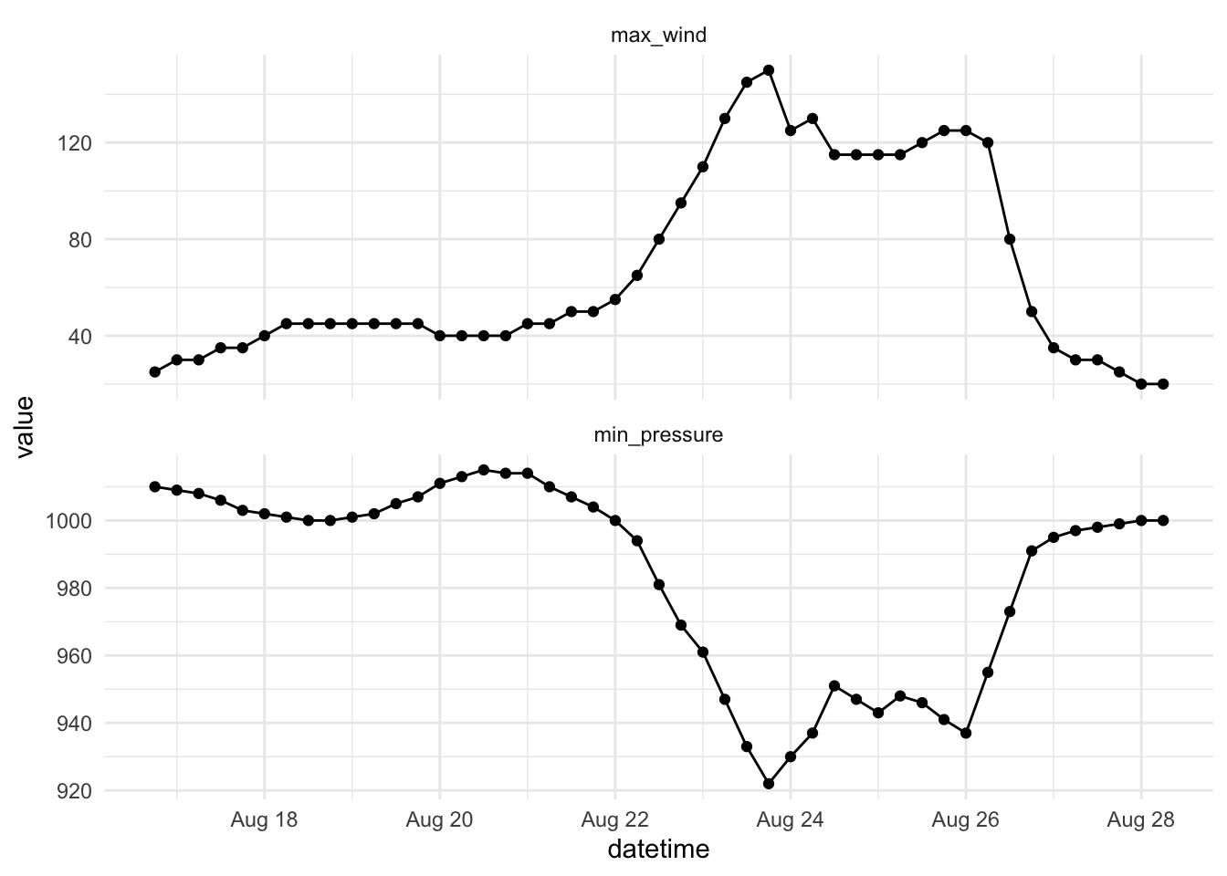
Figure 1.3: Example of how variables in a date-time class can be parsed for sensible axis labels.
1.6.2 Pulling out date and time elements
Once an object is in a date or date-time class (POSIXlt or POSIXct, respectively), there are other functions in the lubridate package you can use to pull certain elements out of it. For example, you can use the functions year, months, mday, wday, yday, weekdays, hour, minute, and second to pull the year, month, month day, etc., of the date. The following code uses the datetime variable in the Hurricane Andrew track data to add new columns for the year, month, weekday, year day, and hour of each observation:
andrew_tracks %>%
  select(datetime) %>%
  mutate(year = year(datetime),
         month = months(datetime),
         weekday = weekdays(datetime),
         yday = yday(datetime),
         hour = hour(datetime)) %>%
  slice(1:3)
# A tibble: 3 x 6
  datetime             year month  weekday  yday  hour
  <dttm>              <dbl> <chr>  <chr>   <dbl> <int>
1 1992-08-16 18:00:00  1992 August Sunday    229    18
2 1992-08-17 00:00:00  1992 August Monday    230     0
3 1992-08-17 06:00:00  1992 August Monday    230     6
This functionality makes it easy to look at patterns in the max_wind value by different time groupings, like weekday and month. For example, the following code puts together some of the dplyr and tidyr data cleaning tools and ggplot2 plotting functions with these lubridate functions to look at the average value of max_wind storm observations by day of the week and by month (Figure 1.4).
check_tracks <- ext_tracks %>%
  select(month, day, hour, year, max_wind) %>%
  unite(datetime, year, month, day, hour) %>%
  mutate(datetime = ymd_h(datetime),
         weekday = weekdays(datetime),
         weekday = factor(weekday, levels = c("Sunday", "Monday",
                                              "Tuesday", "Wednesday",
                                              "Thursday", "Friday",
                                              "Saturday")),
         month = months(datetime),
         month = factor(month, levels = c("April", "May", "June",
                                          "July", "August", "September",
                                          "October", "November",
                                          "December", "January")))

check_weekdays <- check_tracks %>%
  group_by(weekday) %>%
  summarize(ave_max_wind = mean(max_wind),
            .groups = "drop") %>%
  rename(grouping = weekday)
check_months <- check_tracks %>%
  group_by(month) %>%
  summarize(ave_max_wind = mean(max_wind),
            .groups = "drop") %>%
  rename(grouping = month)

a <- ggplot(check_weekdays, aes(x = grouping, y = ave_max_wind)) +
  geom_bar(stat = "identity") + xlab("")
b <- a %+% check_months

library(gridExtra)
grid.arrange(a, b, ncol = 1)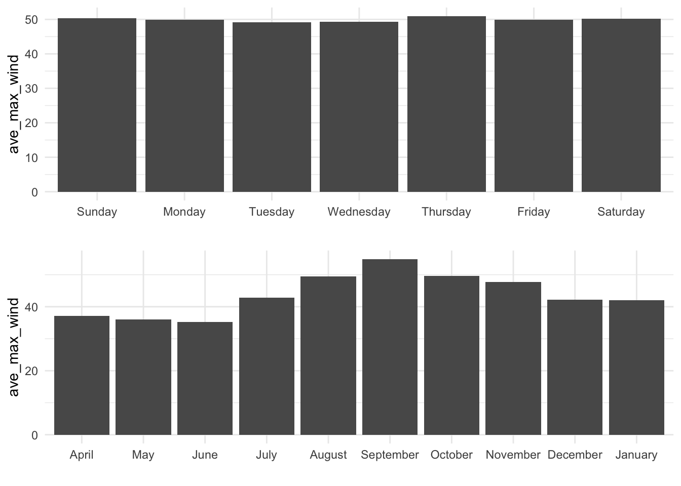
Figure 1.4: Example of using lubridate functions to explore data with a date variable by different time groupings
Based on Figure 1.4, there’s little pattern in storm intensity by day of the week, but there is a pattern by month, with the highest average wind speed measurements in observations in September and neighboring months (and no storm observations in February or March).
There are a few other interesting things to note about this code:
- To get the weekday and month values in the right order, the code uses the
factorfunction in conjunction with thelevelsoption, to control the order in which R sets the factor levels. By specifying the order we want to use withlevels, the plot prints out using this order, rather than alphabetical order (try the code without thefactorcalls for month and weekday and compare the resulting graphs to the ones shown here). - The
grid.arrangefunction, from thegridExtrapackage, allows you to arrange differentggplotobjects in the same plot area. Here, I’ve used it to put the bar charts for weekday (a) and for month (b) together in one column (ncol = 1). - If you ever have
ggplotcode that you would like to re-use for a new plot with a different data frame, you can save a lot of copying and pasting by using the%+%function. This function takes a ggplot object (ain this case, which is the bar chart by weekday) and substitutes a different data frame (check_months) for the original one (check_weekdays), but otherwise maintains all code. Note that we usedrenameto give the x-variable the same name in both datasets so we could take advantage of the%+%function.
1.6.3 Working with time zones
The lubridate package also has functions for handling time zones. The hurricane tracks date-times are, as is true for a lot of weather data, in Coordinated Universal Time (UTC). This means that you can plot the storm track by date, but the dates will be based on UTC rather than local time near where the storm hit. Figure 1.5 shows the location of Hurricane Andrew by date as it neared and crossed the United States, based on date-time observations in UTC.
NOTE: To run the code below, you need a working Google Maps API Key. In order to create an API key, you need to
- Create a Google account (if you do not already have one)
- Goto the Google Maps Platform Console to create an API key
- Enable the Google Maps Static Map API and the Geocoding API for your account
- Copy the Google Maps API key into your
.Renvironfile and store it under the identifierGOOGLEMAPS_API_KEY.
andrew_tracks <- ext_tracks %>%
  filter(storm_name == "ANDREW") %>%
  slice(23:47) %>%
  select(year, month, day, hour, latitude, longitude) %>%
  unite(datetime, year, month, day, hour) %>%
  mutate(datetime = ymd_h(datetime),
         date = format(datetime, "%b %d"))

library(ggmap)

## Need a Google Maps API Key for this to work!
maps_api_key <- Sys.getenv("GOOGLEMAPS_API_KEY")
register_google(key = maps_api_key)

miami <- get_map("miami", zoom = 5)
ggmap(miami) +
  geom_path(data = andrew_tracks, aes(x = -longitude, y = latitude),
            color = "gray", size = 1.1) +
  geom_point(data = andrew_tracks,
             aes(x = -longitude, y = latitude, color = date),
             size = 2)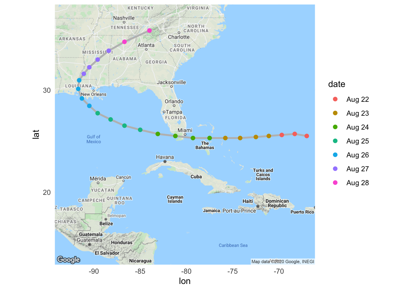
Figure 1.5: Hurricane Andrew tracks by date, based on UTC date times.
To create this plot using local time for Miami, FL, rather than UTC (Figure 1.6), you can use the with_tz function from lubridate to convert the datetime variable in the track data from UTC to local time. This function inputs a date-time object in the POSIXct class, as well as a character string with the time zone of the location for which you’d like to get local time, and returns the corresponding local time for that location.
andrew_tracks <- andrew_tracks %>%
  mutate(datetime = with_tz(datetime, tzone = "America/New_York"),
         date = format(datetime, "%b %d"))

ggmap(miami) +
  geom_path(data = andrew_tracks, aes(x = -longitude, y = latitude),
            color = "gray", size = 1.1) +
  geom_point(data = andrew_tracks,
             aes(x = -longitude, y = latitude, color = date),
             size = 2)
Figure 1.6: Hurricane Andrew tracks by date, based on Miami, FL, local time.
With Figure 1.6, it is clearer that Andrew made landfall in Florida on the morning of August 24 local time.
I> This section has only skimmed the surface of the date-time manipulations you can do with the lubridate package. For more on what this package can do, check out Garrett Grolemund and Hadley Wickham’s article in the Journal of Statistical Software on the package– “Dates and Times Made Easy with lubridate”– or the current package vignette.