4.5 The grid Package

The grid package in R implements the primitive graphical functions that underlie the ggplot2 plotting system. While one typically does not interact directly with the grid package (it is imported by the ggplot2 package), it is necessary to understand some aspects of the grid package in order to build new geoms and graphical elements for ggplot2. In this section we will discuss key elements of the grid package that can be used in extending ggplot2.

While the grid package can be used to produce graphical output directly, it is seldom used for that purpose. Rather, the grid package provides a set of functions and classes that represent graphical objects or grobs, that can be manipulated like any other R object. With grobs, we can manipulate graphical elements (“edit” them) using standard R functions.

4.5.1 Overview of grid graphics

Functions in the ggplot2 package allow extensive customization of many plotting elements. For example, as described in previous sections, you can use ggplot2 functions to change the theme of a plot (and you can also change specific elements of the theme for a plot), to customize the colors used within the plot, and to create faceted “small multiple” graphs. You can even include mathematical annotation on ggplot objects using ggplot2 functions (see https://github.com/tidyverse/ggplot2/wiki/Plotmath for some examples) and change coordinate systems (for example, a pie chart can be created by using polar coordinates on a barchart geom).

Grid graphics is a low-level system for plotting within R and is as a separate system from base R graphics. By “low-level,” we mean that grid graphics functions are typically used to modify very specific elements of a plot, rather than being functions to use for a one-line plotting call. For example, if you want to quickly plot a scatterplot of data, you should use ggplot2, but if you want to create a plot with an inset plot with tilted axis labels, then you may need to go to grid graphics.

The ggplot2 package is built on top of grid graphics, so the grid graphics system “plays well” with ggplot2 objects. In particular, ggplot objects can be added to larger plot output using grid graphics functions, and grid graphics functions can be used to add elements to ggplot objects. Grid graphics functions can also be used to create almost any imaginable plot from scratch. A few other graphics packages, including the lattice package, are also built using grid graphics.

Since it does take more time and code to create plots using grid graphics compared to plotting with ggplot2, it is usually only worth using grid graphics when you need to create a very unusual plot that cannot be created using ggplot2. As people add more geoms and other extensions to ggplot, there are more capabilities for creating customized plots directly in ggplot2 without needing to use the lower-level functions from the grid package. However, they are useful to learn because they provide you the tools to create your own extensions, including geoms.

I> The grid package is now a base package, which means it is installed automatically when you install R. This means you won’t have to install it using install.packages() before you use it. You will, however, have to load the package with library() when you want to use it in an R session.

Grid graphics and R’s base graphics are two separate systems. You cannot easily edit a plot created using base graphics with grid graphics functions. If you have to integrate output from these two systems, you may be able to using the gridBase package, but it will not be as straightforward as editing an object build using grid graphics (including ggplot objects). While we have focused on plotting using ggplot2 in this course, we have covered a few plots created using base R, specifically the maps created by running a plot call on a spatial object, like a SpatialPoints object.

4.5.2 Grobs

The most critical concept of grid graphics to understand for extending ggplot2 it the concept of grobs. Grobs are graphical objects that you can make and change with grid graphics functions. For example, you may create a circle grob or points grobs. Once you have created one or more of these grobs, you can add them to or take them away from larger grid graphics objects, including ggplot objects. These grobs are the actual objects that get printed to a graphics device when you print a grid graphics plot; if you tried to create a grid graphics plot without any grobs, you would get a blank plot.

The grid package has a Grob family of functions that either make or change grobs. If you want to build a custom geom for ggplot that is unusual enough that you cannot rely on inheriting from an existing geom, you will need to use functions from the Grob family of functions to code your geom. You can create a variety of different types of grobs to plot different elements. Possible grobs that can be created using functions in the grid package include circles, rectangles, points, lines, polygons, curves, axes, rasters, segments, and plot frames. You can create grobs using the functions from the *Grob family of functions in the grid package; these functions include circleGrob, linesGrob, polygonGrob, rasterGrob, rectGrob, segmentsGrob, legendGrob, xaxisGrob, and yaxisGrob.

I> Other packages, including the gridExtra package, provide functions that can be used to create addition grobs beyond those provided by the grid package. For example, the gridExtra package includes a function called tableGrob to create a table grob that can be added to grid graphics objects.

Functions that create grobs typically include parameters to specify the location where the grobs should be placed. For example, the pointsGrob function includes x and y parameters, while the segmentsGrob includes parameters for the starting and ending location of each segment (x0, x1, y0, y1).

The grob family of functions also includes a parameter called gp for setting graphical parameters like color, fill, line type, line width, etc., for grob objects. The input to this function must be a gpar object, which can be created using the gpar function. For example, to create a gray circle grob, you could run:

library(grid)
my_circle <- circleGrob(x = 0.5, y = 0.5, r = 0.5,
                        gp = gpar(col = "gray", lty = 3))

Aesthetics that you can set by specifying a gpar object for the gp parameter of a grob include color (col), fill (fill), transparency (alpha), line type (lty), line width (lwd), line end and join styles (lineend and linejoin, respectively), and font elements (fontsize, fontface, fontfamily). See the helpfile for gpar for more on gpar objects.

Once you have created a grob object, you can use the grid.draw function to plot it to the current graphics device. For example, to plot the circle grob we just created, you could run:

grid.draw(my_circle)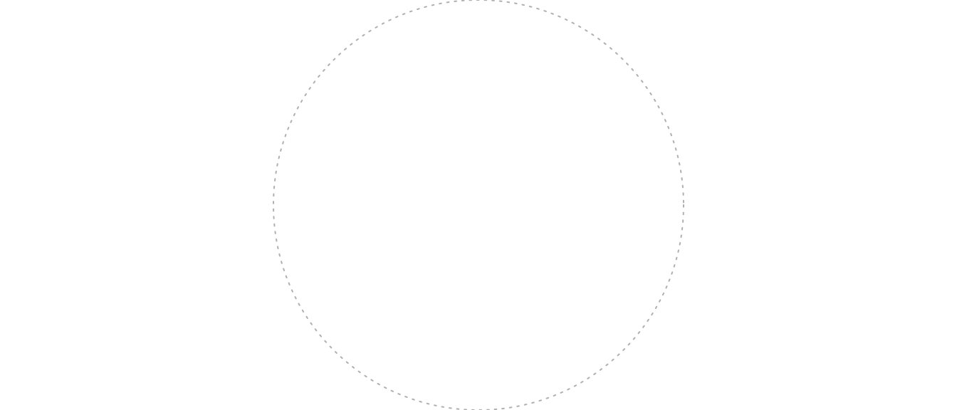

Figure 4.99: Grid circle

In this case, the circle will fill up the full graphics device and will be centered in the middle of the plot region. Later in this subsection, we’ll explain how to use coordinates and coordinate systems to place a grob and how to use viewports to move into subregions of the plotting space.

You can edit a grob after you have drawn it using the grid.edit function. For example, the following code creates a circle grob, draws it, creates and draws a rectangle grob, and then goes back and edits the circle grob within the plot region to change the line type and color (run this code one line at a time within your R session to see the changes). Note that the grob is assigned a name to allow referencing it with the grid.edit call.

my_circle <- circleGrob(name = "my_circle",
                        x = 0.5, y = 0.5, r = 0.5,
                        gp = gpar(col = "gray", lty = 3))
grid.draw(my_circle)

my_rect <- rectGrob(x = 0.5, y = 0.5, width = 0.8, height = 0.3)
grid.draw(my_rect)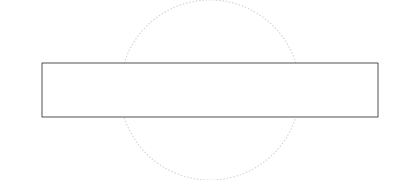

Figure 4.100: Grid objects

grid.edit("my_circle", gp = gpar(col = "red", lty = 1))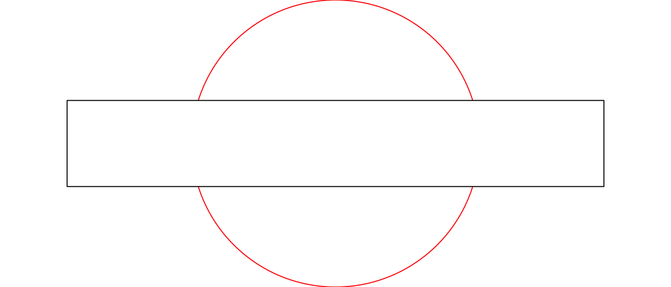

Figure 4.101: Grid objects

As mentioned earlier, ggplot2 was built using the grid system, which means that ggplot objects often integrate well into grid graphics plots. In many ways, ggplot objects can be treated as grid graphics grobs. For example, you can use the grid.draw function from grid to write a ggplot object to the current graphics device:

wc_plot <- ggplot(worldcup, aes(x = Time, y = Passes)) + 
  geom_point()
grid.draw(wc_plot)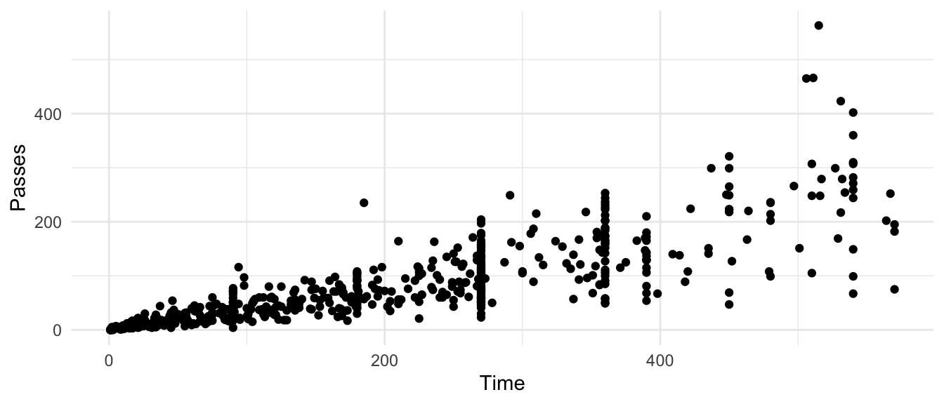

Figure 4.102: Grid scatterplot

This functionality means that ggplot objects can be added to plots with other grobs. For example, once you have defined my_circle and wc_plot using the code above, try running the following code (clear your graphics device first using the broom icon in the RStudio Plots panel):

grid.draw(wc_plot)
grid.draw(my_circle)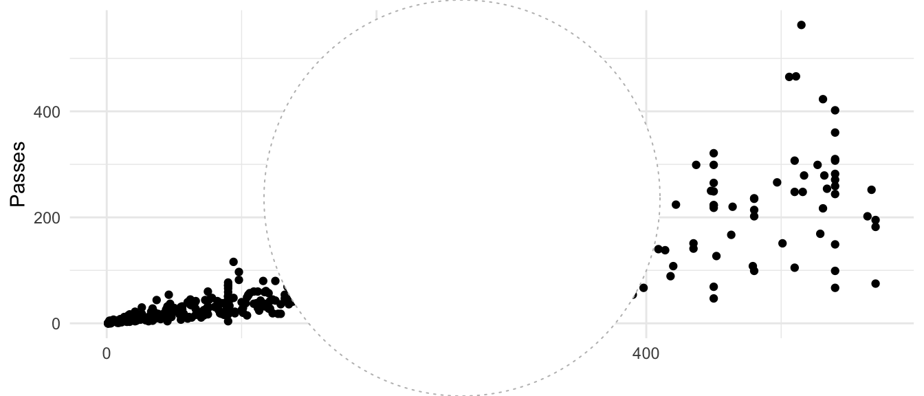

Figure 4.103: Adding ggplot objects to grid plots

In this case, the resulting plot is not very useful, but this functionality will be more interesting once we introduce how to use viewports and coordinate systems.

You can also edit elements of a ggplot object using grid graphics functions. First, you will need to list out all the graphics elements in the ggplot object, so you can find the name of the one you want to change. Then you can use grid.edit to edit that element of the plot.

To find the names of the elements in this ggplot object, first plot the object to RStudio’s graphics device (as done with the last call), then run grid.force, run grid.ls() to find the name of the element you want to change, then use grid.edit to change it. As a note, the exact names of elements will change each time you print out the plot, so you will need to write the grid.edit call based on the grid.ls results for a specific plotting of the ggplot object.

For example, you can run this call to print out the World Cup plot coded earlier and list the names of all elements:

wc_plot
grid.force()
grid.ls()

layout
  background.1-7-10-1
  panel.6-4-6-4
    grill.gTree.1413
      panel.background..rect.1404
      panel.grid.minor.y..polyline.1406
      panel.grid.minor.x..polyline.1408
      panel.grid.major.y..polyline.1410
      panel.grid.major.x..polyline.1412
    NULL
    geom_point.points.1400
    NULL
    panel.border..zeroGrob.1401
  spacer.7-5-7-5
  spacer.7-3-7-3
  spacer.5-5-5-5
  spacer.5-3-5-3
  axis-t.5-4-5-4
  axis-l.6-3-6-3
    axis.line.y..zeroGrob.1432
    axis
      axis.1-1-1-1
        GRID.text.1429
      axis.1-2-1-2
  axis-r.6-5-6-5
  axis-b.7-4-7-4
    axis.line.x..zeroGrob.1425
    axis
      axis.1-1-1-1
      axis.2-1-2-1
        GRID.text.1422
  xlab-t.4-4-4-4
  xlab-b.8-4-8-4
    GRID.text.1416
  ylab-l.6-2-6-2
    GRID.text.1419
  ylab-r.6-6-6-6
  subtitle.3-4-3-4
  title.2-4-2-4
  caption.9-4-9-4

Then, you can change the color of the points to red and the y-axis label to be bold by using grid.edit on those elements (note that if you are running this code yourself, you will need to get the exact names from the grid.ls output on your device):

grid.edit("geom_point.points.1400", gp = gpar(col = "red"))
grid.edit("GRID.text.1419", gp = gpar(fontface = "bold"))

You can use the ggplotGrob function from the ggplot2 package to explicitly make a ggplot grob from a ggplot object.

A gTree grob contains one or more “children” grobs. It can very useful for creating grobs that need to contain multiple elements, like a boxplot, which needs to include a rectangle, lines, and points, or a labeling grob that includes text surrounded by a rectangle. For example, to create a grob that looks like a lollipop, you can run:

candy <- circleGrob(r = 0.1, x = 0.5, y = 0.6)
stick <- segmentsGrob(x0 = 0.5, x1 = 0.5, y0 = 0, y1 = 0.5)
lollipop <- gTree(children = gList(candy, stick))
grid.draw(lollipop)

Figure 4.104: Adding a lollipop

You can use the grid.ls function to list all the children grobs in a gTree:

grid.ls(lollipop)
GRID.gTree.7233
  GRID.circle.7231
  GRID.segments.7232

I> In a later section, we show how to make your own geoms to add to ggplot starting from grid grobs. Bob Rudis has created a geom_lollipop in his ggalt package that allows you to create “lollipop charts” as an alternative to bar charts. For more, see the GitHub repository for ggalt and his blog post on geom_lollipop.

4.5.3 Viewports

Much of the power of grid graphics comes from the ability to move in and out of working spaces around the full graph area. As an example, say you would like to create a map of the states of the US with a small pie chart added at the centroid of each state showing the distribution of population in that state by education level. This kind of plot is where grid graphics shines (although it appears that you now can create such a plot directly in ggplot2). In this case, you want to zoom in at the coordinates of a state centroid, have your own smaller working space at that location, add a pie chart showing data specific to that state within that working space, then zoom out and do the process again for a different state centroid.

In grid graphics, these smaller working spaces within the larger plot are called viewports. Viewports are the plotting windows that you can move into and out of to customize plots using grid graphics. You can navigate to one of the viewports, make some changes, and then pop back up and navigate deeply into another viewport in the plot. In short, viewports provide a way to navigate around and work within different subspaces on a plot.

Using grid graphics, you will create plots by making viewports, navigating into them, writing grobs, and then moving to a different viewport to continue plotting.

To start, you can make a new viewport with the viewport function. For example, to create a viewport in the top right quarter of the full plotting area and write a rounded rectangle and the lollipop grob we defined earlier in this section (we’ve written a rectangle grob before creating a using the viewport, so you can see the area of the full plotting area), you can run:

grid.draw(rectGrob())
sample_vp <- viewport(x = 0.5, y = 0.5, 
                      width = 0.5, height = 0.5,
                      just = c("left", "bottom"))
pushViewport(sample_vp)
grid.draw(roundrectGrob())
grid.draw(lollipop)
popViewport()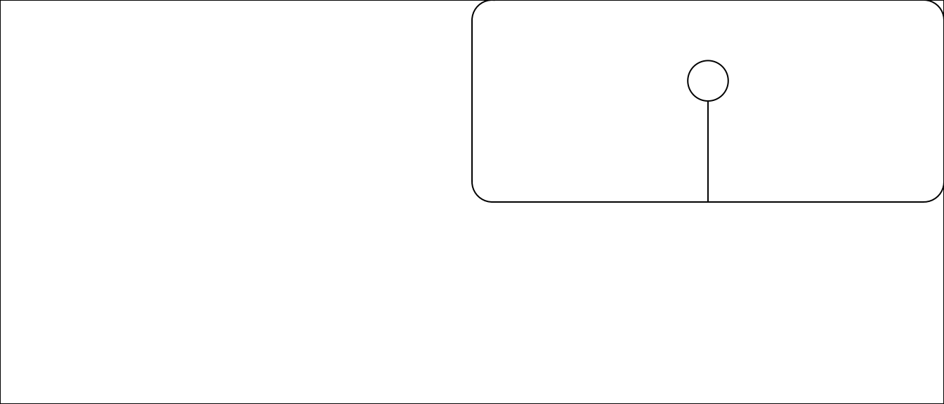

Figure 4.105: Using viewports in grid

This code creates a viewport using the viewport function, navigates into it using pushViewport, writes the grobs using grid.draw, and the navigates out of the viewport using popViewport.

In this code, the x and y parameters of the viewport function specify the viewport’s location, and the just parameter specifies how to justify the viewport in relation to this location. By default, these locations are specified based on a range of 0 to 1 on each side of the plotting area, so x = 0.5 and y = 0.5 specifies the center of the plotting area, while just = c("left", "bottom") specifies that the viewport should have this location at its bottom left corner. If you wanted to place the viewport in the center of the plotting area, for example, you could run:

grid.draw(rectGrob())
sample_vp <- viewport(x = 0.5, y = 0.5, 
                      width = 0.5, height = 0.5,
                      just = c("center", "center"))
pushViewport(sample_vp)
grid.draw(roundrectGrob())
grid.draw(lollipop)
popViewport()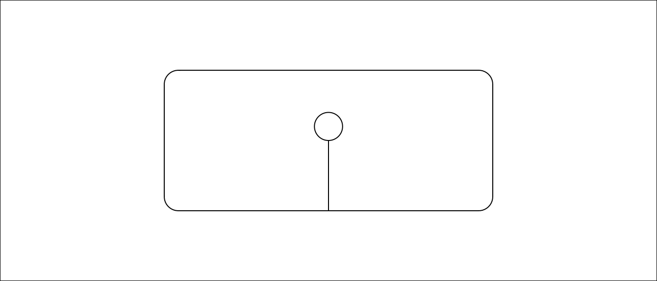

The width and height parameters specify the size of the viewport, again based on default units that 1 is the full width of one side of the plotting area (later in this section, we discuss how to use different coordinate systems). For example, if you wanted to make the viewport smaller, you could run:

grid.draw(rectGrob())
sample_vp <- viewport(x = 0.75, y = 0.75, 
                      width = 0.25, height = 0.25,
                      just = c("left", "bottom"))
pushViewport(sample_vp)
grid.draw(roundrectGrob())
grid.draw(lollipop)
popViewport()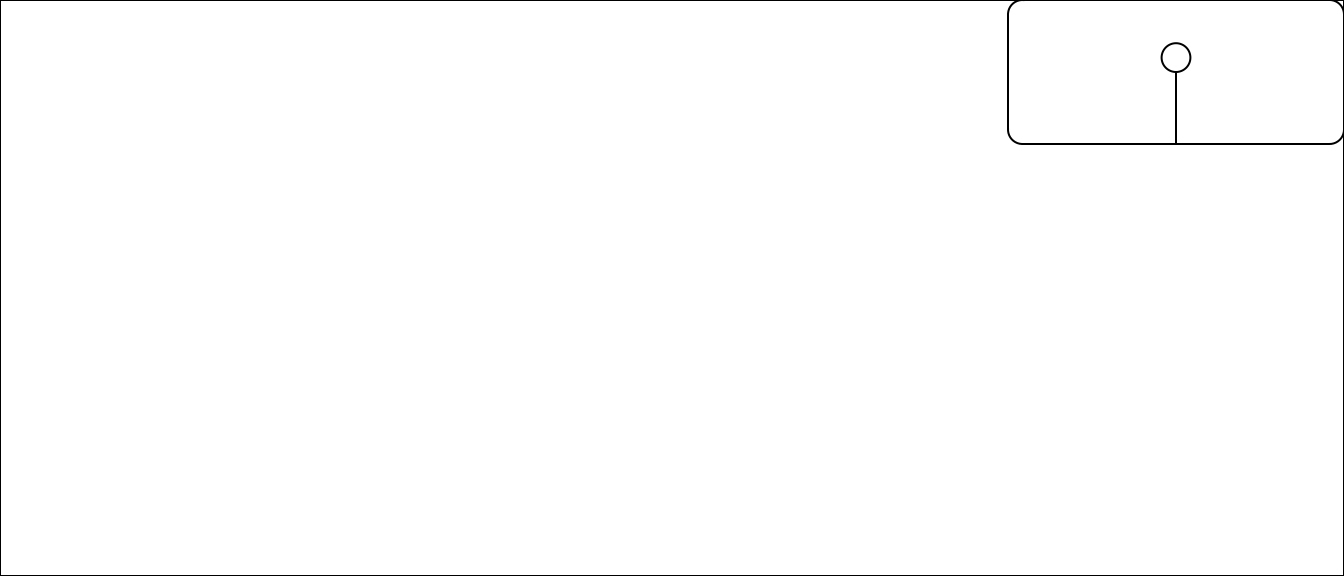

You can only operate in one viewport at a time. Once you are in that viewport, you can write grobs within the viewport. If you want to place the next grob in a different viewport, you will need to navigate out of that viewport before you can do so. Notice that all the previous code examples use popViewport to navigate out of the viewport after writing the desired grobs. We could then create a new viewport somewhere else and write new grobs there:

grid.draw(rectGrob())

sample_vp_1 <- viewport(x = 0.75, y = 0.75, 
                      width = 0.25, height = 0.25,
                      just = c("left", "bottom"))
pushViewport(sample_vp_1)
grid.draw(roundrectGrob())
grid.draw(lollipop)
popViewport()

sample_vp_2 <- viewport(x = 0, y = 0, 
                      width = 0.5, height = 0.5,
                      just = c("left", "bottom"))
pushViewport(sample_vp_2)
grid.draw(roundrectGrob())
grid.draw(lollipop)
popViewport()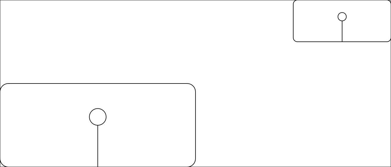

Figure 4.106: Multiple viewports

You can also nest viewports inside each other. In this case, a new viewport is defined relative to the current viewport. For example, if you are in a viewport and position a new viewport at x = 0.5 and y = 0.5, this viewport will be centered in your current viewport rather than in the overall plotting area.

grid.draw(rectGrob())

sample_vp_1 <- viewport(x = 0.5, y = 0.5, 
                      width = 0.5, height = 0.5,
                      just = c("left", "bottom"))
sample_vp_2 <- viewport(x = 0.1, y = 0.1, 
                      width = 0.4, height = 0.4,
                      just = c("left", "bottom"))

pushViewport(sample_vp_1)
grid.draw(roundrectGrob(gp = gpar(col = "red")))
pushViewport(sample_vp_2)
grid.draw(roundrectGrob())
grid.draw(lollipop)
popViewport(2)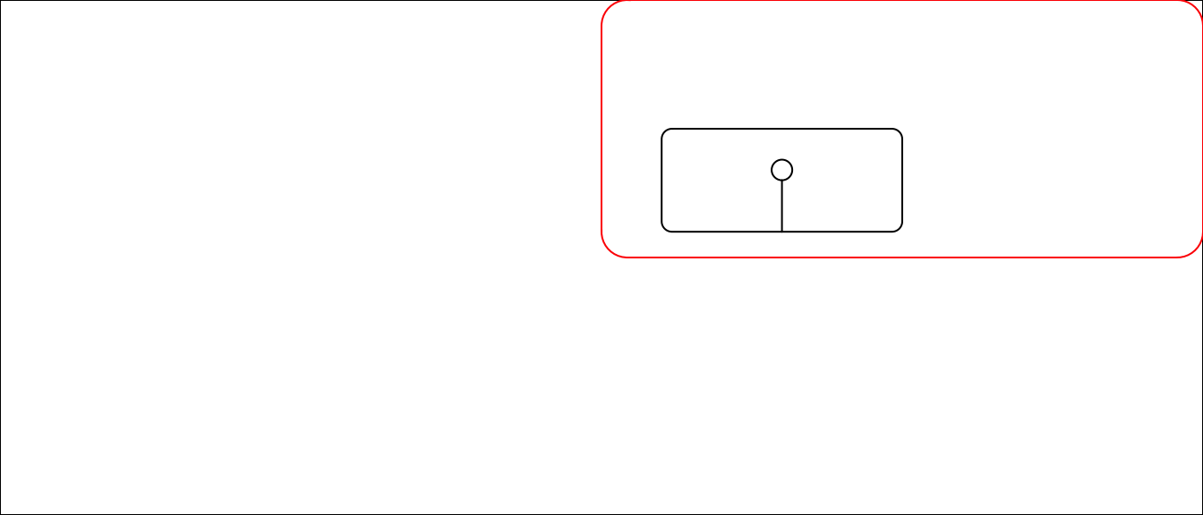

Figure 4.107: Nested viewports

Note that in this code we use the call popViewport(2) to navigate back to the main plotting area. This is because we have navigated down to a viewport within a viewport, so we need to pop up two levels to get out of the viewports.

Given this ability to nest viewports, a grid graphics object can end up with a complex tree of viewports and grobs. Any of these elements can be customized, as long as you can navigate back down to the specific element you want to change.

You can use the grid.ls function to list all the elements of the plot in the current graphics device, if it was created using grid graphics.

grid.draw(rectGrob())

sample_vp_1 <- viewport(x = 0.5, y = 0.5, 
                      width = 0.5, height = 0.5,
                      just = c("left", "bottom"))
pushViewport(sample_vp_1)
grid.draw(roundrectGrob())
grid.draw(lollipop)
popViewport()

grid.ls()
GRID.rect.7246
GRID.roundrect.7247
GRID.gTree.7233
  GRID.circle.7231
  GRID.segments.7232

For ggplot objects, you can also use grid.ls, but you should first run grid.force to set the grobs as they appear in the current graph (or as they will appear when you plot this specific ggplot object), so you can see child grobs in the listing:

worldcup %>%
  ggplot(aes(x = Time, y = Passes)) + 
  geom_point()
grid.force()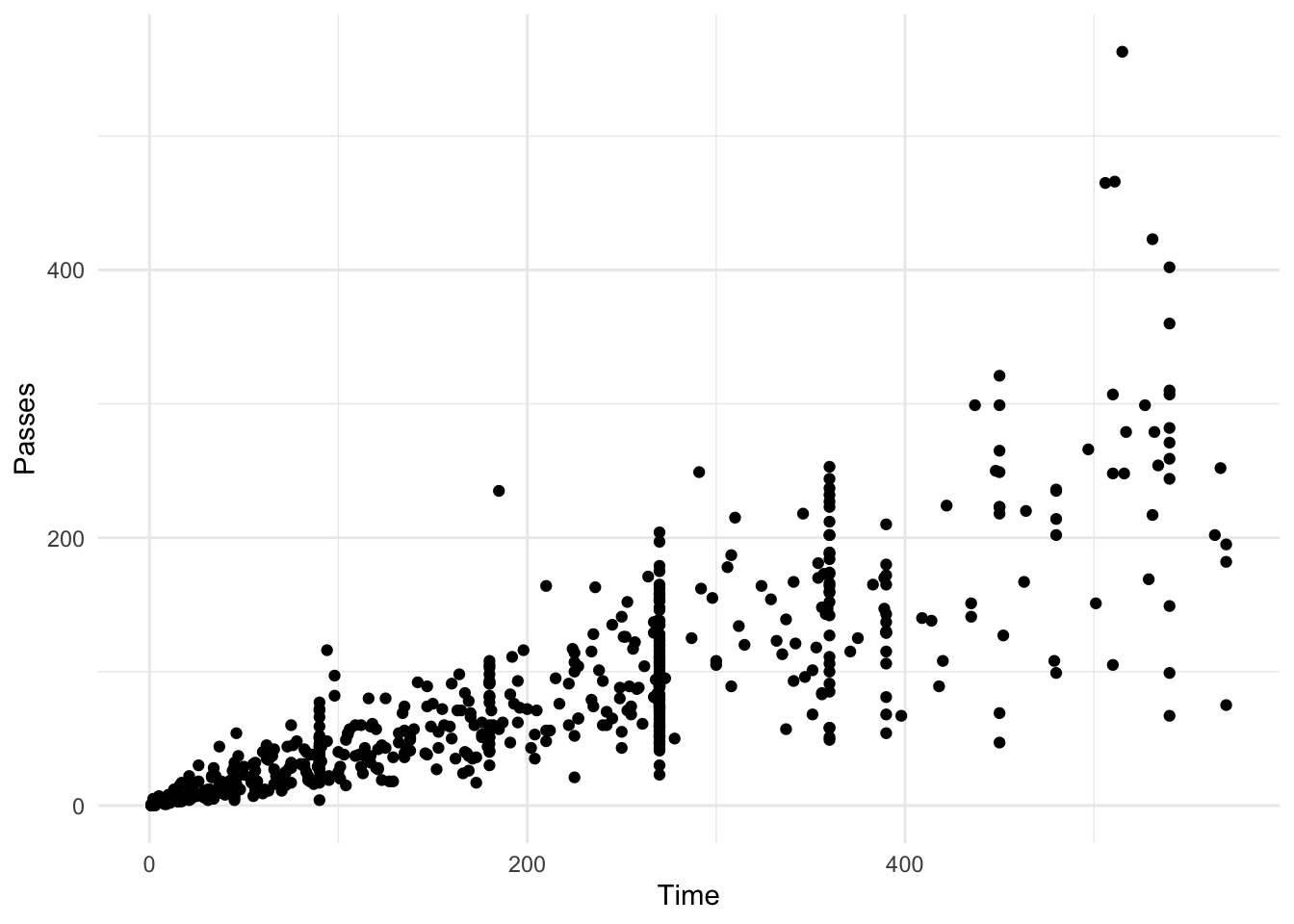

grid.ls()
layout
  background.1-9-12-1
  panel.7-5-7-5
    grill.gTree.7261
      panel.background..zeroGrob.7252
      panel.grid.minor.y..polyline.7254
      panel.grid.minor.x..polyline.7256
      panel.grid.major.y..polyline.7258
      panel.grid.major.x..polyline.7260
    NULL
    geom_point.points.7249
    NULL
    panel.border..zeroGrob.7250
  spacer.8-6-8-6
  spacer.8-4-8-4
  spacer.6-6-6-6
  spacer.6-4-6-4
  axis-t.6-5-6-5
  axis-l.7-4-7-4
    NULL
    axis
      axis.1-1-1-1
        GRID.text.7267
      axis.1-2-1-2
  axis-r.7-6-7-6
  axis-b.8-5-8-5
    NULL
    axis
      axis.1-1-1-1
      axis.2-1-2-1
        GRID.text.7264
  xlab-t.5-5-5-5
  xlab-b.9-5-9-5
    GRID.text.7270
  ylab-l.7-3-7-3
    GRID.text.7273
  ylab-r.7-7-7-7
  subtitle.4-5-4-5
  title.3-5-3-5
  caption.10-5-10-5
  tag.2-2-2-2

You can use ggplot objects in plots with viewports. For example, you can use the following code to add an inset map for the map we created earlier in this section of Baltimore County and Baltimore City in Maryland. The following code creates ggplot objects with the main plot and the inset map and uses viewports to create a plot showing both. Note that in the viewport we’ve added two rectangle grobs, one in white with some transparency to provide the background of the map inset, and one with no fill and color set to black to provide the inset border.

balt_counties <- map_data("county", region = "maryland") %>%
  mutate(our_counties = subregion %in% c("baltimore", "baltimore city"))
balt_map <- get_map("Baltimore County", zoom = 10) %>%
  ggmap(extent = "device") + 
  geom_polygon(data = filter(balt_counties, our_counties == TRUE),
               aes(x = long, y = lat, group = group),
               fill = "red", color = "darkred", alpha = 0.2)
maryland_map <- balt_counties %>%
  ggplot(aes(x = long, y = lat, group = group, fill = our_counties)) + 
  geom_polygon(color = "black") + 
  scale_fill_manual(values = c("white", "darkred"), guide = FALSE) + 
  theme_void() + 
  coord_map()

grid.draw(ggplotGrob(balt_map))
md_inset <- viewport(x = 0, y = 0, 
                     just = c("left", "bottom"),
                     width = 0.35, height = 0.35)
pushViewport(md_inset)
grid.draw(rectGrob(gp = gpar(alpha = 0.5, col = "white")))
grid.draw(rectGrob(gp = gpar(fill = NA, col = "black")))
grid.draw(ggplotGrob(maryland_map))
popViewport()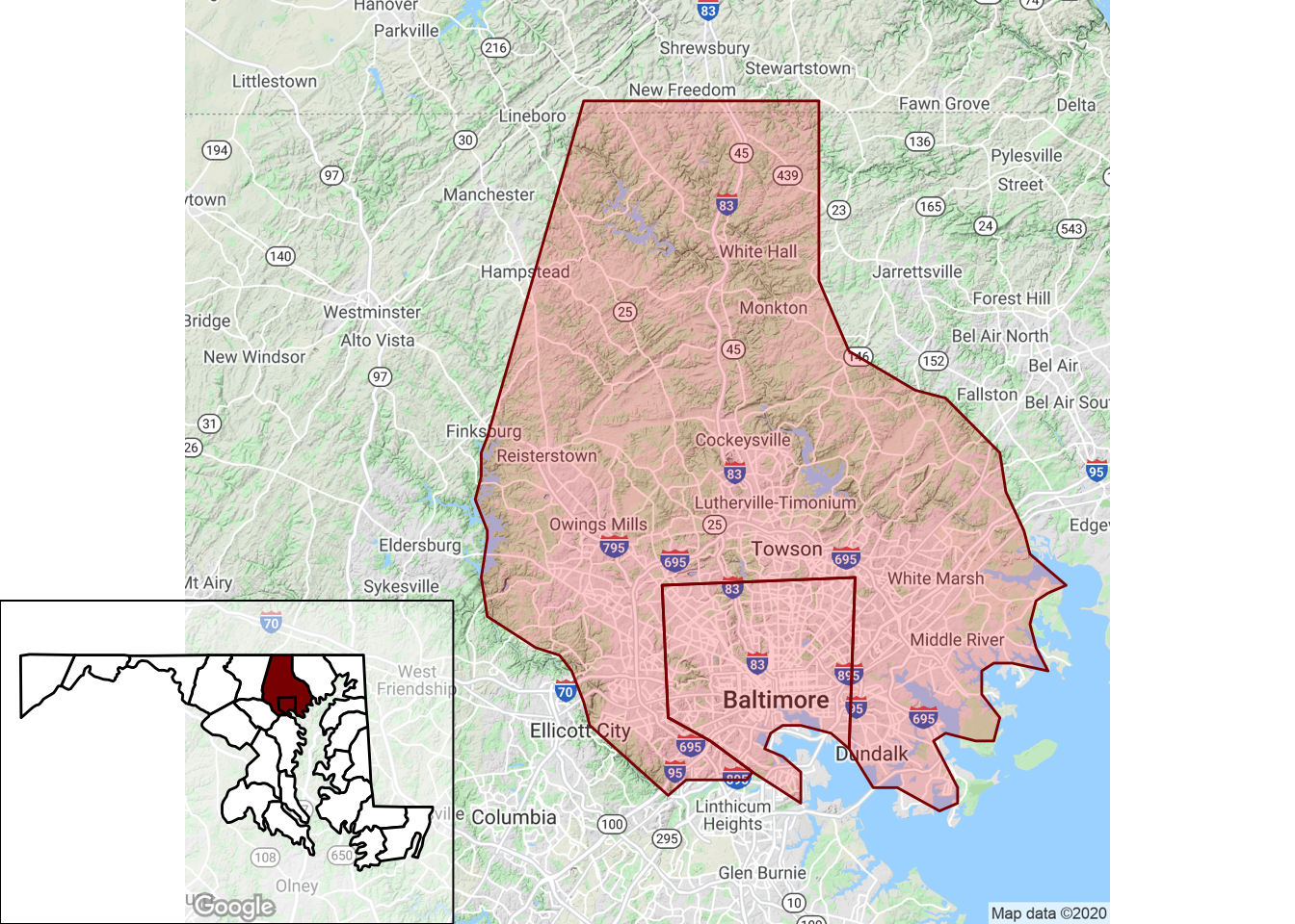

Figure 4.108: Adding an inset map

4.5.4 Grid graphics coordinate systems

Once you have created a grob and moved into the viewport in which you want to plot it, you need a way to specify where in the viewport to write the grob. The numbers you use to specify x- and y-placements for a grob will depend on the coordinate system you use. In grid graphics, you have a variety of options for the units to use in this coordinate system, and picking the right units for this coordinate system will make it much easier to create the plot you want.

There are several units that can be used for coordinate systems, and you typically will use different units to place objects. For example, you may want to add points to a plot based on the current x- and y-scales in that plot region, in which case you can use native units. The native unit is often the most useful when creating extensions for ggplot2, for example. The npc units are also often useful in designing new plots– these set the x- and y-ranges to go from 0 to 1, so you can use these units if you need to place an object in, for example, the exact center of a viewport (c(0.5, 0.5) in npc units), or create a viewport in the top right quarter of the plot region. Grid graphics also allows the use of some units with absolute values, including inches (inches), centimeters (cm), and millimeters (mm).

You can specify the coordinate system you would like to use when placing an object by with the unit function (unit([numeric vector], units = "native")). For example, if you create a viewport with the x-scale going from 0 to 100 and the y-scale going from 0 to 10 (specified using xscale and yscale in the viewport function), you can use native when drawing a grob in that viewport to base the grob position on these scale values.

ex_vp <- viewport(x = 0.5, y = 0.5, 
                  just = c("center", "center"),
                  height = 0.8, width = 0.8,
                  xscale = c(0, 100), yscale = c(0, 10))
pushViewport(ex_vp)
grid.draw(rectGrob())
grid.draw(circleGrob(x = unit(20, "native"), y = unit(5, "native"),
                     r = 0.1, gp = gpar(fill = "lightblue")))
grid.draw(circleGrob(x = unit(85, "native"), y = unit(8, "native"),
                     r = 0.1, gp = gpar(fill = "darkred")))
popViewport()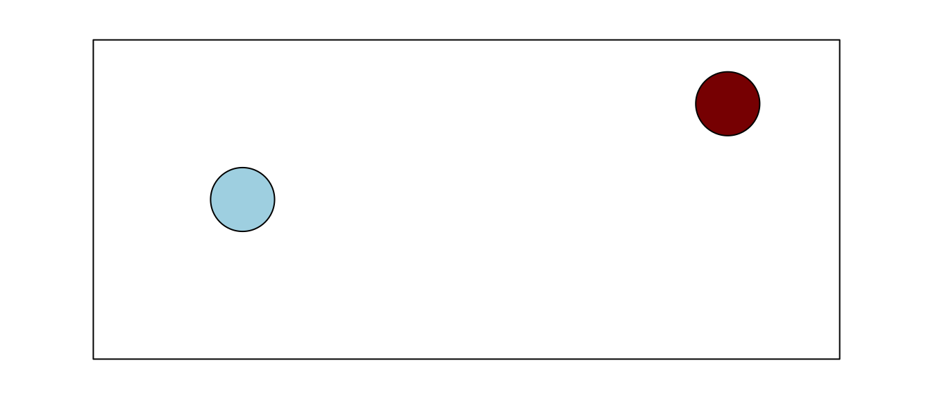

Figure 4.109: Specifying coordinate systems

4.5.5 The gridExtra package

The gridExtra package provides useful extensions to the grid system, with an emphasis on higher-level functions to work with grid graphic objects, rather than the lower-level utilities in the grid package that are used to create and edit specific lower-level elements of a plot. This package has particularly useful functions that allow you to arrange and write multiple grobs to a graphics device and to include tables in grid graphics objects.

The grid.arrange function from the gridExtra package makes it easy to create a plot with multiple grid objects plotted on it. For example, you can use it to write out one or more grobs you’ve created to a graphics device:

library(gridExtra)
grid.arrange(lollipop, circleGrob(),
             rectGrob(), lollipop, 
             ncol = 2)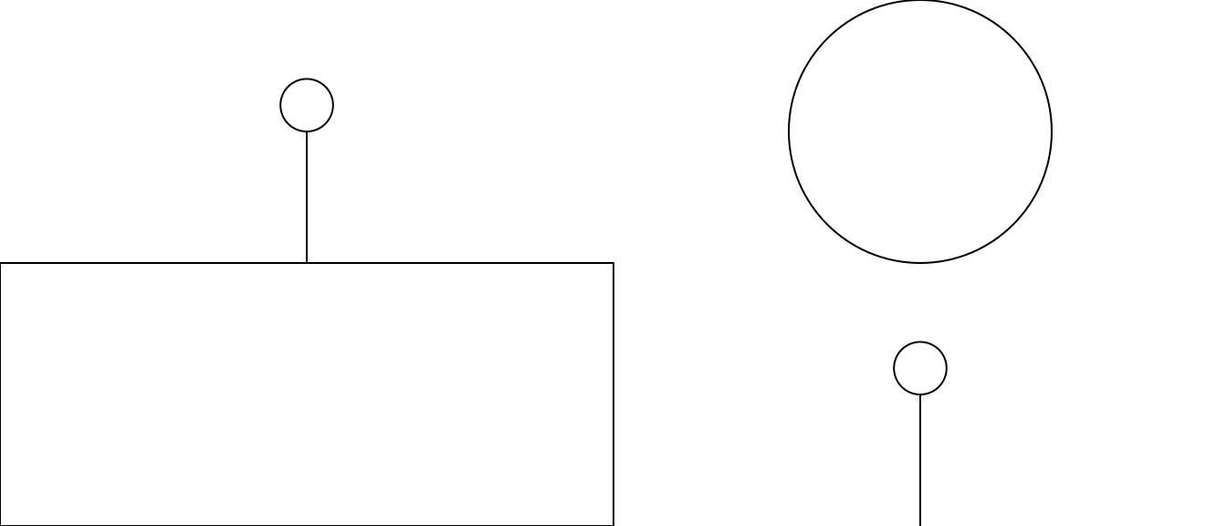

Figure 4.110: Using grid.arrange()

Note that this code is being used to arrange both grobs that were previously created and saved to an R object (the lollipop grob created in earlier code in this section) and grobs that are created within the grid.arrange call (the grobs created with circleGrob and rectGrob). The ncol parameter is used to specify the number of columns to include in the output.

Because ggplot2 was built on grid graphics, you can also use this function to plot multiple ggplot objects to a graphics device. For example, say you wanted to create a plot that has two plots based on the World Cup data side-by-side. To create this plot, you can assign the ggplot objects for each separate graph to objects in your R global environment (time_vs_shots and player_positions in this example), and then input these objects to a grid.arrange call:

time_vs_shots <- ggplot(worldcup, aes(x = Time, y = Shots)) + 
  geom_point()
player_positions <- ggplot(worldcup, aes(x = Position)) + 
  geom_bar()

grid.arrange(time_vs_shots, player_positions, ncol = 2)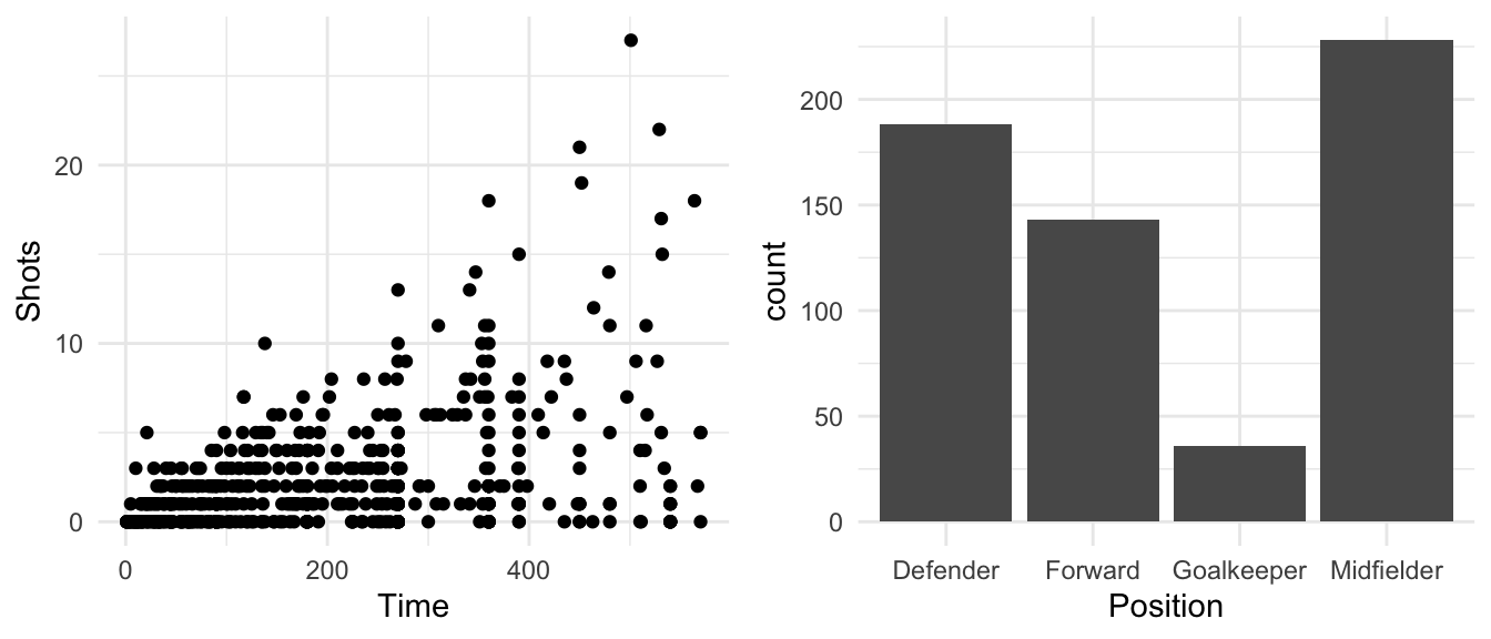

Figure 4.111: Using grid.arrange()

You can use the layout_matrix parameter to specify different layouts. For example, if you want the scatterplot to take up one-third of the plotting area and the bar chart to take up two-thirds, you could specify that with a matrix with one “1” (for the first plot) and two “2s,” all in one row:

grid.arrange(time_vs_shots, player_positions,
             layout_matrix = matrix(c(1, 2, 2), ncol = 3))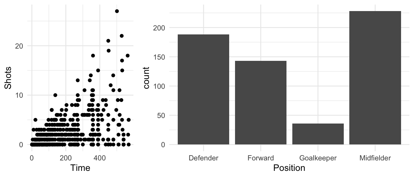

Figure 4.112: Arranging multiple plots in a matrix

You can fill multiple rows in the plotting device. To leave a space blank, use NA in the layout matrix at that positions. For example:

grid.arrange(time_vs_shots, player_positions,
             layout_matrix = matrix(c(1, NA, NA, NA, 2, 2), 
                                    byrow = TRUE, ncol = 3))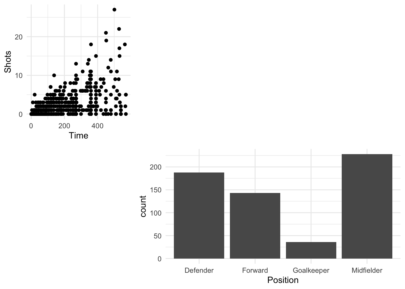

Figure 4.113: Adding blank space to a matrix of plots

The gridExtra also has a function, tableGrob, that facilitates in adding tables to grid graphic objects. For example, to add a table with the average time and shots for players on the top four teams in the 2010 World Cup, you can create a table grob using tableGrob and then add it to a larger plot created using grid graphics:

worldcup_table <- worldcup %>%
  filter(Team %in% c("Germany", "Spain", "Netherlands", "Uruguay")) %>%
  group_by(Team) %>%
  dplyr::summarize(`Average time` = round(mean(Time), 1),
                   `Average shots` = round(mean(Shots), 1)) %>%
  tableGrob()
`summarise()` ungrouping output (override with `.groups` argument)

grid.draw(ggplotGrob(time_vs_shots))
wc_table_vp <- viewport(x = 0.22, y = 0.85, 
                        just = c("left", "top"),
                        height = 0.1, width = 0.2)
pushViewport(wc_table_vp)
grid.draw(worldcup_table)
popViewport()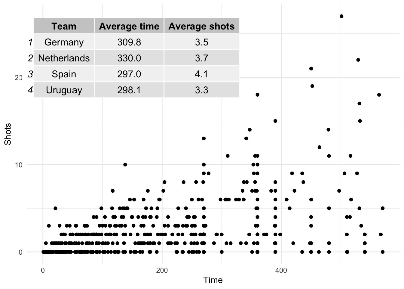

These tables can be customized with different trend and can be modified by adding other grob elements (for example, to highlight certain cells). To find out more, see the vignette for table grobs.

4.5.6 Find out more about grid graphics

Grid graphics provide an extensive graphics system that can allow you to create almost any plot you can imagine in R. In this section, we have only scraped the surface of the grid graphics system, so you might want to study grid graphics in greater depth, especially if you often need to create very tailored, unusual graphs.

There are a number of resources you can use to learn more about grid graphics. The most comprehensive is the R Graphics book by Paul Murrell, the creator of grid graphics. This book is now in its second edition, and its first edition was written before ggplot2 became so popular. It is worth try to get the second edition, which includes some content specifically on ggplot2 and how that package relates to grid graphics. The vignettes that go along with the grid package are also by Paul Murrell and give a useful introduction to grid graphics, and the vignettes for the gridExtra package are also a useful next step for finding out more.

• Links to pdfs of vignettes for the grid graphics package are available at https://stat.ethz.ch/R-manual/R-devel/library/grid/doc/index.html
• Links to pdfs of vignettes for the gridGraphics package are available on the package’s CRAN page: https://cran.r-project.org/web/packages/gridExtra/index.html