2.3 Functional Programming
The learning objectives of the section are:
- Describe functional programming concepts
- Write functional programming code using the
purrrpackage
2.3.1 What is Functional Programming?
Functional programming is a programming philosophy based on lambda calculus. Lambda calculus was created by Alonzo Church, the PhD adviser to Alan Turing who is known for his role in cracking the encryption of the Nazi’s Enigma machine during World War Two. Functional programming has been a popular approach ever since it helped bring down the Third Reich.
Functional programming concentrates on four constructs:
- Data (numbers, strings, etc)
- Variables (function arguments)
- Functions
- Function Applications (evaluating functions given arguments and/or data)
By now you’re used to treating variables inside of functions as data, whether they’re values like numbers and strings, or they’re data structures like lists and vectors. With functional programming you can also consider the possibility that you can provide a function as an argument to another function, and a function can return another function as its result.
If you’ve used functions like sapply() or args() then it’s easy to imagine
how functions as arguments to other functions can be used. In the case of
sapply() the provided function is applied to data, and in the case of args()
information about the function is returned. What’s rarer to see is a function
that returns a function when it’s evaluated. Let’s look at a small example of
how this can work:
adder_maker <- function(n){
  function(x){
    n + x
  }
}

add2 <- adder_maker(2)
add3 <- adder_maker(3)

add2(5)
[1] 7
add3(5)
[1] 8
In the example above the function adder_maker() returns a function with no
name. The function returned adds n to its only argument x.
2.3.2 Core Functional Programming Functions
There are groups of functions that are essential for functional programming.
In most cases they take a function and a data structure as arguments, and that
function is applied to that data structure in some way. The purrr library
contains many of these functions and we’ll be using it throughout this section.
Function programming is concerned mostly with lists and vectors. I may refer to
just lists or vectors, but you should know that what applies for lists generally
applies for vectors and vice-versa.
2.3.2.1 Map
The map family of functions applies a function to the elements of a data
structure, usually a list or a vector. The function is evaluated once for each
element of the vector with the vector element as the first argument to the
function. The return value is the same kind if data structure (a list or vector)
but with every element replaced by the result of the function being evaluated
with the corresponding element as the argument to the function. In the purrr
package the map() function returns a list, while the map_lgl(), map_chr(),
and map_dbl() functions return vectors of logical values, strings, or numbers
respectively. Let’s take a look at a few examples:
library(purrr)

map_chr(c(5, 4, 3, 2, 1), function(x){
  c("one", "two", "three", "four", "five")[x]
})
[1] "five"  "four"  "three" "two"   "one"

map_lgl(c(1, 2, 3, 4, 5), function(x){
  x > 3
})
[1] FALSE FALSE FALSE  TRUE  TRUE
Think about evaluating each function above with just one of the arguments in the specified numeric vector, and then combining all of those function results into one vector.
The map_if() function takes as its arguments a list or vector containing data,
a predicate function, and then a function to be applied. A predicate function is
a function that returns TRUE or FALSE for each element in the provided list
or vector. In the case of map_if(): if the predicate functions evaluates to
TRUE, then the function is applied to the corresponding vector element,
however if the predicate function evaluates to FALSE then the function is not
applied. The map_if() function always returns a list, so I’m piping the
result of map_if() to unlist() so it look prettier:
map_if(1:5, function(x){
              x %% 2 == 0
            },
            function(y){
              y^2
            }) %>% unlist()
[1]  1  4  3 16  5
Notice how only the even numbers are squared, while the odd numbers are left alone.
The map_at() function only applies the provided function to elements of a
vector specified by their indexes. map_at() always returns a list so like
before I’m piping the result to unlist():
map_at(seq(100, 500, 100), c(1, 3, 5), function(x){
  x - 10
}) %>% unlist()
[1]  90 200 290 400 490
Like we expected to happen the providied function is only applied to the first, third, and fifth element of the vector provided.
In each of the examples above we have only been mapping a function over one
data structure, however you can map a function over two data structures with
the map2() family of functions. The first two arguments should be two vectors
of the same length, followed by a function which will be evaluated with an
element of the first vector as the first argument and an element of the second
vector as the second argument. For example:
map2_chr(letters, 1:26, paste)
 [1] "a 1"  "b 2"  "c 3"  "d 4"  "e 5"  "f 6"  "g 7"  "h 8"  "i 9"  "j 10"
[11] "k 11" "l 12" "m 13" "n 14" "o 15" "p 16" "q 17" "r 18" "s 19" "t 20"
[21] "u 21" "v 22" "w 23" "x 24" "y 25" "z 26"
The pmap() family of functions is similar to map2(), however instead of
mapping across two vectors or lists, you can map across any number of lists.
The list argument is a list of lists that the function will map over, followed
by the function that will applied:
pmap_chr(list(
  list(1, 2, 3),
  list("one", "two", "three"),
  list("uno", "dos", "tres")
), paste)
[1] "1 one uno"    "2 two dos"    "3 three tres"
Mapping is a powerful technique for thinking about how to apply computational operations to your data.
2.3.2.2 Reduce
List or vector reduction iteratively combines the first element of a vector
with the second element of a vector, then that combined result is combined with
the third element of the vector, and so on until the end of the vector is
reached. The function to be applied should take at least two arguments.
Where mapping returns a vector or a list, reducing should return a
single value. Some examples using reduce() are illustrated below:
reduce(c(1, 3, 5, 7), function(x, y){
  message("x is ", x)
  message("y is ", y)
  message("")
  x + y
})
x is 1
y is 3

x is 4
y is 5

x is 9
y is 7

[1] 16
On the first iteration x has the value 1 and y has the value 3, then the
two values are combined (they’re added together). On the second iteration x
has the value of the result from the first iteration (4) and y has the value of
the third element in the provided numeric vector (5). This process is repeated
for each iteration. Here’s a similar example using string data:
reduce(letters[1:4], function(x, y){
  message("x is ", x)
  message("y is ", y)
  message("")
  paste0(x, y)
})
x is a
y is b

x is ab
y is c

x is abc
y is d

[1] "abcd"
By default reduce() starts with the first element of a vector and then the
second element and so on. In contrast the reduce_right() function starts with
the last element of a vector and then proceeds to the second to last element of
a vector and so on:
reduce_right(letters[1:4], function(x, y){
  message("x is ", x)
  message("y is ", y)
  message("")
  paste0(x, y)
})
Warning: `reduce_right()` is soft-deprecated as of purrr 0.3.0.
Please use the new `.dir` argument of `reduce()` instead.

  # Before:
  reduce_right(1:3, f)

  # After:
  reduce(1:3, f, .dir = "backward")  # New algorithm
  reduce(rev(1:3), f)                # Same algorithm as reduce_right()

This warning is displayed once per session.
x is d
y is c

x is dc
y is b

x is dcb
y is a

[1] "dcba"
2.3.2.3 Search
You can search for specific elements of a vector using the has_element() and
detect() functions. has_element() will return TRUE if a specified element
is present in a vector, otherwise it returns FALSE:
has_element(letters, "a")
[1] TRUE
has_element(letters, "A")
[1] FALSE
The detect() function takes a vector and a predicate function as arguments and
it returns the first element of the vector for which the predicate function
returns TRUE:
detect(20:40, function(x){
  x > 22 && x %% 2 == 0
})
[1] 24
The detect_index() function takes the same arguments, however it returns the
index of the provided vector which contains the first element that satisfies
the predicate function:
detect_index(20:40, function(x){
  x > 22 && x %% 2 == 0
})
[1] 5
2.3.2.4 Filter
The group of functions that includes keep(), discard(), every(), and
some() are known as filter functions. Each of these functions takes a vector
and a predicate function. For keep() only the elements of the vector that
satisfy the predicate function are returned while all other elements are
removed:
keep(1:20, function(x){
  x %% 2 == 0
})
 [1]  2  4  6  8 10 12 14 16 18 20
The discard() function works similarly, it only returns elements that don’t
satisfy the predicate function:
discard(1:20, function(x){
  x %% 2 == 0
})
 [1]  1  3  5  7  9 11 13 15 17 19
The every() function returns TRUE only if every element in the vector
satisfies the predicate function, while the some() function returns TRUE if
at least one element in the vector satisfies the predicate function:
every(1:20, function(x){
  x %% 2 == 0
})

some(1:20, function(x){
  x %% 2 == 0
})
2.3.2.5 Compose
Finally, the compose() function combines any number of functions into one
function:
n_unique <- compose(length, unique)
# The composition above is the same as:
# n_unique <- function(x){
#   length(unique(x))
# }

rep(1:5, 1:5)
 [1] 1 2 2 3 3 3 4 4 4 4 5 5 5 5 5

n_unique(rep(1:5, 1:5))
[1] 5
2.3.3 Functional Programming Concepts
2.3.3.1 Partial Application
Partial application of functions can allow functions to behave a little like
data structures. Using the partial() function from the purrr package you
can specify some of the arguments of a function, and then partial() will return
a function that only takes the unspecified arguments. Let’s take a look at a
simple example:
library(purrr)

mult_three_n <- function(x, y, z){
  x * y * z
}

mult_by_15 <- partial(mult_three_n, x = 3, y = 5)

mult_by_15(z = 4)
[1] 60
By using partial application you can bind some data to the arguments of a function before using that function elsewhere.
2.3.3.2 Side Effects
Side effects of functions occur whenever a function interacts with the “outside
world” – reading or writing data, printing to the console, and displaying a
graph are all side effects. The results of side effects are one of the main
motivations for writing code in the first place! Side effects can be tricky to
handle though, since the order in which functions with side effects are executed
often matters and there are variables that are external to the program (the
relative location of some data). If you want to evaluate a function across
a data structure you should use the walk() function from purrr. Here’s a
simple example:
library(purrr)

walk(c("Friends, Romans, countrymen,",
       "lend me your ears;",
       "I come to bury Caesar,",
       "not to praise him."), message)
Friends, Romans, countrymen,
lend me your ears;
I come to bury Caesar,
not to praise him.
2.3.3.3 Recursion
Recursion is very powerful tool, both mentally and in software development, for solving problems. Recursive functions have two main parts: a few easy to solve problems called “base cases,” and then a case for more complicated problems where the function is called inside of itself. The central philosophy of recursive programming is that problems can be broken down into simpler parts, and then combining those simple answers results in the answer to a complex problem.
Imagine you wanted to write a function that adds together all of the numbers in a vector. You could of course accomplish this with a loop:
vector_sum_loop <- function(v){
  result <- 0
  for(i in v){
    result <- result + i
  }
  result
}

vector_sum_loop(c(5, 40, 91))
[1] 136
You could also think about how to solve this problem recursively. First ask yourself: what’s the base case of finding the sum of a vector? If the vector only contains one element, then the sum is just the value of that element. In the more complex case the vector has more than one element. We can remove the first element of the vector, but then what should we do with the rest of the vector? Thankfully we have a function for computing the sum of all of the elements of a vector because we’re writing that function right now! So we’ll add the value of the first element of the vector to whatever the cumulative sum is of the rest of the vector. The resulting function is illustrated below:
vector_sum_rec <- function(v){
  if(length(v) == 1){
    v
  } else {
    v[1] + vector_sum_rec(v[-1])
  }
}

vector_sum_rec(c(5, 40, 91))
[1] 136
Another useful exercise for thinking about applications for recursion is computing the Fibonacci sequence. The Fibonacci sequence is a sequence of integers that starts: 0, 1, 1, 2, 3, 5, 8 where each proceeding integer is the sum of the previous two integers. This fits into a recursive mental framework very nicely since each subsequent number depends on the previous two numbers.
Let’s write a function to computues the nth digit of the Fibonacci sequence such that the first number in the sequence is 0, the second number is 1, and then all proceeding numbers are the sum of the n - 1 and the n - 2 Fibonacci number. It is immediately evident that there are three base cases:
- n must be greater than 0.
- When n is equal to 1, return 0.
- When n is equal to 2, return 1.
And then the recursive case:
- Otherwise return the sum of the n - 1 Fibonacci number and the n - 2 Fibonacci number.
Let’s turn those words into code:
fib <- function(n){
  stopifnot(n > 0)
  if(n == 1){
    0
  } else if(n == 2){
    1
  } else {
    fib(n - 1) + fib(n - 2)
  }
}

fib(1)
[1] 0
fib(2)
[1] 1
fib(3)
[1] 1
fib(4)
[1] 2
fib(5)
[1] 3
fib(6)
[1] 5
fib(7)
[1] 8

map_dbl(1:12, fib)
 [1]  0  1  1  2  3  5  8 13 21 34 55 89
Looks like it’s working well! There is one optimization that we could apply here
which comes up in recursive programming often. When you execute the function
fib(6), within that function you’ll execute fib(5) and fib(4). Then within
the execution of fib(5), fib(4) will be executed again. An illustration of
this phenomenon is below:
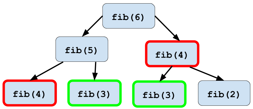
Figure 2.1: Memoization of fib() function
This duplication of computation slows down your program significantly as you calculate larger numbers in the Fibonacci sequence. Thankfully you can use a technique called memoization in order to speed this computation up. Memoization stores the value of each calculated Fibonacci number in table so that once a number is calculated you can look it up instead of needing to recalculate it!
Below is an example of a function that can calculate the first 25 Fibonacci
numbers. First we’ll create a very simple table which is just a vector
containing 0, 1, and then 23 NAs. First the fib_mem() function will check
if the number is in the table, and if it is then it is returned. Otherwise the
Fibonacci number is recursively calculated and stored in the table. Notice that
we’re using the complex assignment operator <<- in order to modify the table
outside the scope of the function. You’ll learn more about the complex operator
in the section titled Expressions & Environments.
fib_tbl <- c(0, 1, rep(NA, 23))

fib_mem <- function(n){
  stopifnot(n > 0)

  if(!is.na(fib_tbl[n])){
    fib_tbl[n]
  } else {
    fib_tbl[n - 1] <<- fib_mem(n - 1)
    fib_tbl[n - 2] <<- fib_mem(n - 2)
    fib_tbl[n - 1] + fib_tbl[n - 2]
  }
}

map_dbl(1:12, fib_mem)
 [1]  0  1  1  2  3  5  8 13 21 34 55 89
It works! But is it any faster than the original fib()? Below I’m going to use
the microbenchmark package in order assess whether fib() or fib_mem() is
faster:
library(purrr)
library(microbenchmark)
library(tidyr)
library(magrittr)
library(dplyr)

fib_data <- map(1:10, function(x){microbenchmark(fib(x), times = 100)$time})
names(fib_data) <- paste0(letters[1:10], 1:10)
fib_data <- as.data.frame(fib_data)

fib_data %<>%
  gather(num, time) %>%
  group_by(num) %>%
  summarise(med_time = median(time))

memo_data <- map(1:10, function(x){microbenchmark(fib_mem(x))$time})
names(memo_data) <- paste0(letters[1:10], 1:10)
memo_data <- as.data.frame(memo_data)

memo_data %<>%
  gather(num, time) %>%
  group_by(num) %>%
  summarise(med_time = median(time))

plot(1:10, fib_data$med_time, xlab = "Fibonacci Number", ylab = "Median Time (Nanoseconds)",
     pch = 18, bty = "n", xaxt = "n", yaxt = "n")
axis(1, at = 1:10)
axis(2, at = seq(0, 350000, by = 50000))
points(1:10 + .1, memo_data$med_time, col = "blue", pch = 18)
legend(1, 300000, c("Not Memoized", "Memoized"), pch = 18,
       col = c("black", "blue"), bty = "n", cex = 1, y.intersp = 1.5)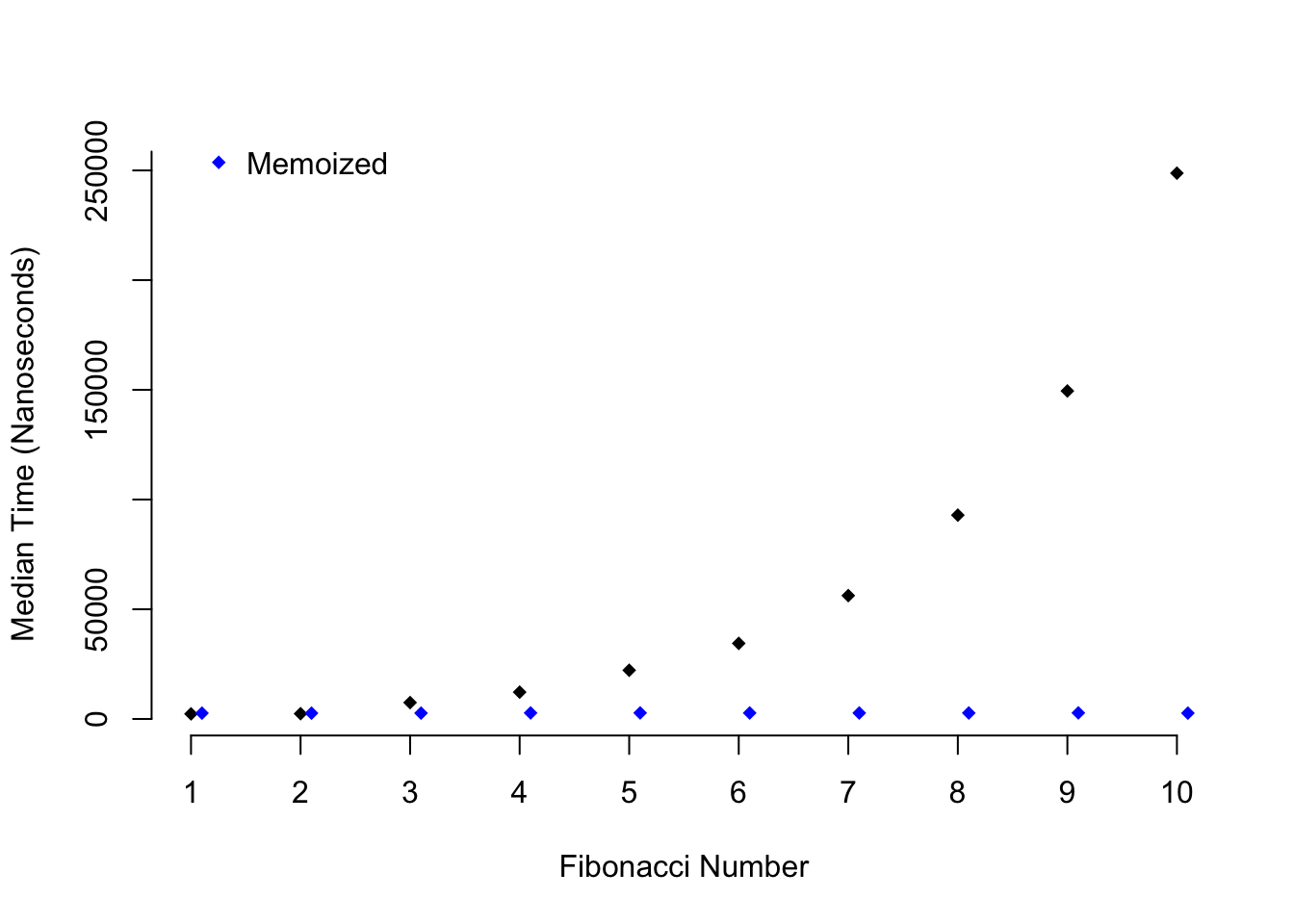
Figure 2.2: Speed comparison of memoization
As you can see as higher Fibonacci numbers are calculated the time it takes to
calculate a number with fib() grows exponentially, while the time it takes
to do the same task with fib_mem() stays constant.
2.3.4 Summary
- Functional programming is based on lambda calculus.
- This approach concentrates on data, variables, functions, and function applications.
- It’s possible for functions to be able to return other functions.
- The core functional programming concepts can be summarized in the following categories: map, reduce, search, filter, and compose.
- Partial application of functions allows functions to be used like data sctructures.
- Side effects are difficult to debug although they motivate a huge fraction of computer programming.
- The most important part of understanding recursion is understanding recursion.